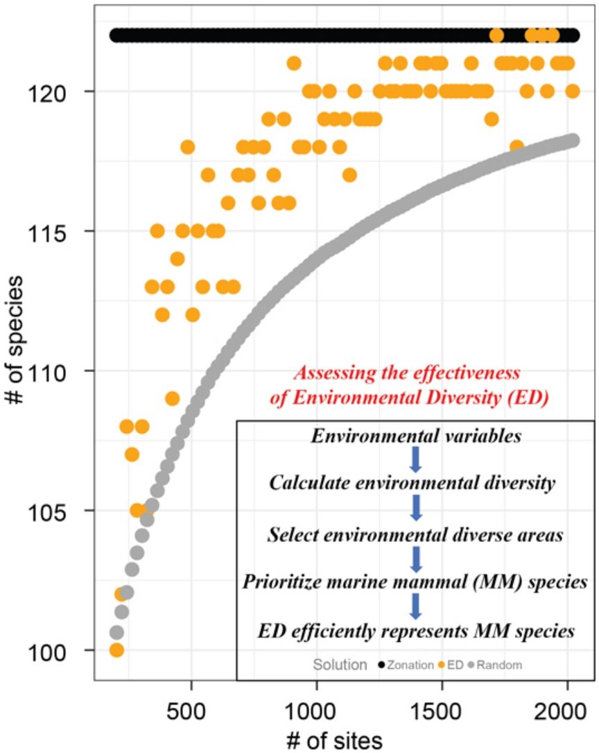
Surrogates are used in conservation planning to select sites to represent species when information about species’ geographical distributions is insufficient. Many surrogates for biodiversity have used biotic (e.g., vegetation assemblages) or biogeographic distributions of a group of species (e.g., birds) that are easier to inventory than more cryptic species of interest. Because knowledge of species geographical distributions is mostly limited, environmental diversity (ED), an approach that uses environmental dissimilarity between sites to select areas for conservation, is a promising alternative surrogacy strategy. While studies in the terrestrial realms justify further investigations of the effectiveness of ED as a surrogate to determine conservation priority of sites, ours represents a significant expansion of this focus to consider the marine realm. In this study, we defined environmental space using nine variables and evaluated ED as a surrogate of global marine mammal species. We found that ED is an effective surrogacy strategy for marine mammals: sites selected to span environmental diversity represented 61% more marine mammals, on average, than a random subset of sites. Although the effectiveness of ED has been demonstrated in previous studies of terrestrial vertebrates, we believe this is the first time ED is assessed as a surrogate in marine systems at the global scale. Our findings suggest that ED may also be useful to prioritize sites for conservation of other marine taxa.
Systematic conservation planning aims to prioritize areas for conservation action, such that the greatest biodiversity is represented while minimizing implementation costs (Rodrigues and Brooks, 2007; Moilanen et al., 2009). To select sites that efficiently represent species, conservation scientists and biogeographers rank sites by complementarity; that is, their ability to add species to the set of species already represented in a set of notionally conserved sites. Thus, sites are prioritized for conservation by preferentially selecting sites with higher numbers of unprotected species. The resulting set of sites represent many more species than if sites had been selected using species richness alone (Kirkpatrick, 1983; Csuti et al., 1997; Albuquerque and Beier, 2015a, b, and papers cited therein). If all sites have been inventoried for species of interest, highly complementary sites can be selected using integer programming (Haight and Snyder, 2009), or by using heuristic algorithms such as Zonation — a reserve-selection software (Moilanen et al., 2014).
Because of the limited knowledge about species and their distributions, conservation planners and biogeographers often use surrogates, such as terrestrial land cover types (Hunter, 1991), well-mapped taxa (Lewandowski et al., 2010), or environmental variables (Faith and Walker, 1996) to prioritize sites for conservation. Abiotic variables (e.g., temperature and topography) have been used to define surrogates for terrestrial (Faith and Walker, 1996; Beier and Albuquerque, 2015; Albuquerque and Beier, 2018) and marine (McArthur et al., 2020; Sutcliffe et al., 2015) biodiversity, and in each case, the surrogates identified sites with high complementarity.
One approach to using abiotic factors as a surrogate is environmental diversity (ED). ED organizes sites in continuous multidimensional environmental space that is assumed to be correlated to species assemblage space, and then uses a p-median algorithm to select sites that span the environmental space (Faith and Walker, 1996; Faith, 2003). The p-median approach starts by creating a uniform grid of hypothetical demand points across the ordination space, and then selects the subset of sites that minimize the distance (in raw multivariate space or ordination space) from each demand point to the nearest selected site (Faith and Walker, 1996; Faith, 2003; Hortal et al., 2009; Beier and Albuquerque, 2015). Another ED approach, Maxdisp (Engelbrecht et al., 2016), does not use demand points, but instead selects the sites with the highest sum of squares of distances among all pairs of selected sites. Engelbrecht et al. (2016) and Albuquerque and Beier (2018) concluded that Maxdisp was at least as effective as continuous p-median in selecting sites that efficiently represent species and has the advantage of faster and simpler computation.
Previous studies in the terrestrial realm have reported that ED is a highly effective surrogacy strategy of plants and vertebrates in tropical and temperate regions (Beier et al., 2015; Albuquerque and Beier, 2018). These findings justify further studies as to the effectiveness of ED as a surrogacy strategy to determine the conservation priority of sites. ED can be particularly meaningful in areas of the world where knowledge of species geographical distributions is most limited, such as tropical regions that might be experiencing rapid biodiversity loss (Pimm, 2000). The present study represents an important expansion of this focus to consider the marine realm. If effective, ED would be especially useful because most ocean areas have not been inventoried for marine mammals and other taxa (Schipper et al., 2008; Mora et al., 2011; Magera et al., 2013).
In marine systems, Sutcliffe et al. (2015) studied how well abiotic variables represented species belonging to a network of reserves in an Australian inter-reef system and found that abiotic information can help design marine reserves. If our hypothesis that ED is an effective surrogacy strategy for marine mammal representation is supported, it would suggest that ED could be used in marine systems as an alternative strategy whenever biological information is limited or lacking. Subsequent studies can then test if ED can also be an efficient surrogacy strategy for other marine taxa. Otherwise, negative results would suggest that although ED is an effective surrogacy strategy in the terrestrial context, it might not be equally applied to the marine landscape, at least in the case of marine mammals. In addition to testing the efficiency of ED as a surrogacy strategy for marine mammals, we also investigated whether the choice of oceanographic variables could affect its effectiveness (Albuquerque and Beier, 2018).
Materials and methodsData preparationWe obtained range maps depicting the distribution of 123 marine mammals from the International Union for the Conservation of Nature (IUCN) Red List Spatial Data database (IUCN, 2021). We processed these range maps using the R package letsR (Vilela and Villalobos, 2015) to generate presence/absence values for each 1° grid cell of the world’s oceans (N = 46,130). We excluded species that occur only in freshwater or are listed as Extinct by the IUCN. Species listed as Not Evaluated (NE) by the IUCN were also not part of our study because there are no range maps available for them.
We conducted separate analyses for 7 subsets or groups of the 123 marine mammals, plus an eighth group that included all species. Two subsets were related to use of land: Fully-aquatic (FA; n = 87 cetaceans and sirenians) or Non-fully aquatic (semiaquatic) (NFA; n = 36 pinnipeds and fissipeds). Three groups related to migratory status: Migratory (MI; n = 37), Non-migratory (NMI; n = 52) or Unknown migratory status (UNK; n = 29). There were too few nomadic species (n = 5) for a separate analysis. Finally, we evaluated ED separately for threatened species (TR; n = 52) and species listed as Least Concern (Non-threatened species or NTR; n = 71). The TR group included species listed as Critically Endangered (CR; n = 3), Endangered (EN; n = 17), Vulnerable (VU; n = 13), Near Threatened (NT; n = 9), and Data Deficient (DD; n = 10). We included DD species in the TR group because Parsons (2016) argued that most DD cetaceans (all DD species are cetaceans) are likely to be threatened, and larger proportions of marine mammals than terrestrial mammals are threatened (Schipper et al., 2008). We also included NT as threatened because NT species are likely to become qualified as threatened in the near future (IUCN, 2012) (Table S1).
For each of the 46,130 1° marine cells or study sites, we considered nine environmental variables expected to affect species distributions at the global extent. Variables were obtained from the World Ocean Atlas (WOA, Boyer et al., 2018). The WOA is a collection of oceanographic variables aimed at depicting the ocean profile data (Garcia et al., 2019). Variables included objectively analyzed annual mean surface values for temperature, salinity, dissolved oxygen, percent oxygen saturation, apparent oxygen utilization, silicate, phosphate, and nitrate from the National Centers for Environmental Information (NOAA, Boyer et al., 2018). We also obtained gridded bathymetric (depth) values for each 1° cell from the Global Ocean and Land Terrain models (GEBCO 30 arc-second grid, GEBCO, 2014).
Measuring complementarityComplementarity provides widely-used values that represent optimal solutions for species in the least number of sites (see e.g., Williams et al., 1996; Albuquerque and Beier, 2015a; Veach et al., 2017). We used the core-area function of the reserve-selection software Zonation (Moilanen et al., 2014) to produce a hierarchical ranking of conservation priorities based on complementarity of every 1° marine cell on Earth for each marine mammal group, based on their distribution maps. Zonation is deterministic and produces a complementarity-based ranking of conservation values over the entire landscape.
Measuring environmental diversity (ED)We used the Maxdisp ED approach (Engelbrecht et al., 2016) and two sets of environmental variables for selecting environmentally diverse sites. The first set encompassed all oceanographic variables (EDall). The second set included temperature, bathymetry and salinity (EDsel); variables known to be related to conservation priority for marine mammals at a global extent (Astudillo-Scalia and Albuquerque, 2020). Maxdisp uses a Euclidean environmental distance matrix among the grid cells (sites) and the inverse of the square of distances between sites to calculate environmental dissimilarities between sites and to select sites maximally dispersed in the environmental space (Engelbrecht et al., 2016). After excluding the cells with missing environmental data, we used 40,401 cells in the analyses.
We used the Species Accumulation Index, SAI (Ferrier and Watson, 1997; Rodrigues and Brooks, 2007) to evaluate the ability of EDall and EDsel to identify sites that most efficiently represent species across 91 targets, ranging from 0.1 to 5.0% (by 0.05 increments) of the most environmentally diverse sites. SAI measures surrogacy values and compares the performance of the surrogate (EDall and EDsel) to the optimum/near optimum result (Zonation) and the randomly-selected sites result. SAI is expressed by: (S-R)/(O-R), where S is the number of species represented in sites with the highest predicted complementarity ranks, O is the maximum number of species that can be represented in the same number of sites (based on complementarity values), and R is the number of species represented in the same number of randomly selected sites. SAI is scaled –∞ to 1; negative SAI indicates a worse than random result, 0 indicates random performance, and positive SAI is a measure of surrogate efficiency. For example, SAI of 0.8 indicates that ED is 80% as effective as having full knowledge of where species occur in its ability to improve on random selection of sites.
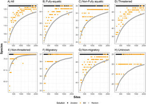
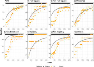
ResultsFor all eight groups and all percentages of sites prioritized (targets), Zonation solutions represented many more species than the same number of randomly-selected sites (Figs. 1 and 2). In general, sites prioritized by the EDall approach represented more species than occurred in randomly selected sites for most datasets (Fig. 1). Random solutions were relatively more efficient at lower targets (Fig. 1). On the other hand, EDsel generally represented significantly fewer species than the Zonation and random solutions (Fig. 2).
Number of marine mammal species represented at least once in sites selected by environmental diversity (EDall), and species represented at least once in sites selected by Zonation, compared to the number of species represented in an equal number of randomly selected sites. ED was calculated using all oceanographic variables. Curves are represented for eight marine mammal groups: (A) all species, (B) fully-aquatic, (C) non-fully aquatic, (D) threatened, (E) non-threatened, (F) migratory, (G) non-migratory, and (H) unknown migratory status.
Number of species represented at least once in sites selected by environmental diversity (EDsel), and species represented at least once in sites selected by Zonation, compared to the number of species represented in an equal number of randomly selected sites. ED was calculated from selected variables (temperature, bathymetry and salinity). Curves are represented for eight marine mammal groups: (A) all species, (B) fully-aquatic, (C) non-fully aquatic, (D) threatened, (E) non-threatened, (F) migratory, (G) non-migratory, and (H) unknown migratory status.
The effectiveness of EDall and EDsel as surrogates for species representation varied across groups. On average across all marine mammal groups and targets, EDall solutions were 61% as effective as Zonation solutions in improving on random selection of sites. EDall represented significantly more species than randomly selected sites for groups Migratory and Non-threatened (mean SAI 0.75 and 0.72, respectively). The lowest efficiency in represented marine mammals was observed for Non-migratory and Non-fully aquatic marine mammals (mean SAI 0.47 and 0.53, respectively). For EDsel, the effectiveness was much lower, except for Threatened species (Table 1). SAI values ranged from -6.0 (Non-migratory) to 0.68 (Threatened). Most SAI values for EDsel, are negative, indicating a performance that is worse than random solutions (Table 1).
Species accumulation indices (SAI) values of environmental diversity (ED) calculated from oceanographic variables. SAI values are represented by the mean across 91 spatial prioritization targets. The confidence level (95%) is also displayed. All variables include mean surface values for temperature, salinity, dissolved oxygen, percent oxygen saturation, apparent oxygen utilization, silicate, phosphate, nitrate, and bathymetry. Selected variables include mean surface values for temperature, bathymetry and salinity.
| Marine Mammal Groups | Variables | |
|---|---|---|
| All | Selected | |
| All species (ALL) | 0.560 (0.05) | −0.316 (0.09) |
| Fully aquatic (FA) | 0.596 (0.05) | 0.026 (0.09) |
| Non-fully aquatic (NFA) | 0.525 (0.06) | −0.732 (0.11) |
| Threatened, NT & DD (TR) | 0.559 (0.05) | 0.682 (0.09) |
| Non-threatened (NTR) | 0.719 (0.17) | −0.568 (0.10) |
| Migratory (MI) | 0.746 (0.08) | 0.002 (0.06) |
| Non-migratory (NMI) | 0.467 (0.06) | −6.007 (0.83) |
| Unknown migratory status (UNK) | 0.703 (0.07) | −0.248 (0.10) |
While the efficacy of ED has been tested in the terrestrial realm (Faith and Walker, 1996; Faith, 2003, 2011, Faith et al., 1996, 2004, Beier and Albuquerque, 2015; Engelbrecht et al., 2016; Albuquerque and Beier, 2018), this study provides a comprehensive assessment of the effectiveness of ED as a surrogate of marine mammal groups. Even though Species Accumulation Index (SAI) values differed among groups, our results suggest that ED is close to complementarity-based models for two of the datasets we tested (Non-threatened and Migratory; Table 1). Potentially, the reason for these observed differences in efficiency is that ED assumes that all species have a unimodal distribution in environmental space (Beier and Albuquerque, 2016), congruent with findings of studies in geographical space (e.g., Brown and Thatje, 2014). However, some marine mammal species deviate from this pattern in geographical space (e.g., migrating species such as humpback whales have a trimodal distribution, with seasonal presence in tropical/subtropical regions and the poles), which might be affecting the performance of the model. Further studies are required to better understand the cause of these patterns. The efficiency of ED depends on the set of environmental variables used to define environmental space (Table 1) and the fraction of the landscape prioritized (Fig. 1). Results of the two ED models in our study suggest that including variables that are related to primary productivity (even when they are not related to marine mammals themselves; e.g., oxygen-related variables, phosphate, and nitrate), has a significant impact on the effectiveness of the ED model. This is likely due to the relationship between marine mammal distribution and primary productivity. For example, Roman and McCarthy (2010) showed that marine mammal fecal plumes can increase primary productivity by contributing an important source of nitrogen close to the surface, and that regions with higher marine mammal densities tend to have higher levels of productivity.
We found that EDall provides an abiotic surrogate that is on average 61% as effective as known distribution maps. In a recent meta-analysis, Beier et al. (2015) reviewed 622 evaluations of the effectiveness of abiotic surrogates in representing species in terrestrial ecosystems and reported that the use of abiotic surrogates represented plants and vegetation types relatively well. Beier and Albuquerque (2015) tested the efficiency of ED in eight terrestrial datasets and showed that ED was 42% as effective as having knowledge of species distributions. Sutcliffe et al. (2015) evaluated the use of abiotic domains to measure the efficacy of different marine reserve systems in representing species for conservation purposes and reported that abiotic domains performed substantially better than random solutions.
As previously mentioned, the high efficiency of ED as a surrogate is linked to the variables used to define the environmental space and to the way ED selects sites for conservation. Abiotic data, and particularly ED, is an efficient surrogate of biotic representation because it selects sites to optimally span environmental space without the arbitrary constraints of binning methods, and because abiotic conditions are often associated with biogeographical patterns of plant and animal species richness, beta diversity, and patterns of sites complementarity (e.g., Currie, 1991; Hawkins et al., 2003; Field et al., 2005; Gaston et al., 2007; Albuquerque and Beier, 2015a). These studies suggest that energy and climate limit species richness over broad geographic extents (Hawkins et al., 2003 and references therein). An important assumption of using ED is that the values of oceanographic variables in a site reflect conditions experienced by marine species. Tittensor et al. (2010) investigated the global patterns and predictors of marine biodiversity and reported that temperature or kinetic energy plays a key role in structuring cross-taxon marine biodiversity. As indicated by the high efficiency of ED in identifying sites that represented species efficiently, our results show that variables related to diversity and complementarity can be used as abiotic surrogates to represent species in the marine realm. This follows the premise that areas with higher environmental diversity can host a greater diversity of species by providing a wider range of environmental conditions or niche space.
Additionally, our findings suggest that different species ought to be managed separately, and that each marine mammal group and environmental variables must be tested on a case-by-case scenario to determine the best abiotic surrogates to represent each species and/or groups. For example, results show that Non-threatened and Migratory species are the best represented by the ED model, while the worst groups represented by this model were Non-fully aquatic and Non-migratory (Table 1).
While we agree that results show that biotic informed solutions are still preferred if the distribution of species is well known, we also show that ED produces reliable solutions for marine mammals (Table 1). In an absence of knowledge about their geographical distribution (such as potential changes in their future distributions due to climate change; Silber et al., 2017), ED could provide the efficiency to meet conservation targets and help design alternative conservation areas, without having to wait for updated distribution maps. Considering that only a small fraction of biodiversity has been described or inventoried (Brown and Lomolino, 1998), and IUCN range maps should not be interpreted at spatial resolution finer than 1-degree cells (Hurlbert and Jetz, 2007), surrogacy strategies, such as ED, are needed for many taxa, especially at the fine spatial resolutions used for real world conservation planning. Since ED needs only abiotic data to select environmental diverse sites, and considering that abiotic data are widely available at finer and coarser resolutions, ED could represent an alternative to determine conservation priority of sites in places where the biographic distribution is lacking, and inventories are limited by budget constraints.
In conclusion, we found that ED could be an effective surrogacy strategy for marine mammals. This is the first study assessing the performance of ED as a surrogate of marine mammal biodiversity representation at the global scale. We propose that our results justify further studies on how ED can be used in applied conservation of marine species by complementing the available biotic information and thus increasing the overall tests of the effectiveness of the surrogates. This is in alignment with the findings by Rodrigues and Brooks (2007) and Sutcliffe et al. (2015), who reported that biologically informed environmental surrogates, those that incorporated biological variables to develop their models, improved the efficiency of abiotic data as a surrogate of biodiversity.
Additionally, we must highlight that the results of our study are in a theoretical framework and therefore not yet ready to be applied in conservation of marine mammals. Range maps often overestimate the presence of species (Hurlbert and Jetz, 2007), and this overestimation may affect conclusions in the identification of efficacy of ED. To make our results more applicable to conservation action, biotic data comprising species-specific life history information such as population density estimates per site, minimum home range data, use of areas and seasonality (i.e., feeding areas versus breeding areas, especially in the case of migratory species), minimum coverage required for effective conservation outcomes (as representation by at least one cell in our model might not be adequate for some species), and other logistical information should all be determined and incorporated into our results. Nonetheless, because these factors are required in the implementation of a marine protected area even if site prioritization is calculated based on entirely biotic metrics such as species richness, we believe that our work as it stands already represents an improvement on site prioritization by complementing available biotic information even when it is scarce.
In the future, when biological information is available, biologically-informed multivariate procedures such as gradient forests (Ellis et al., 2012) and generalized dissimilarity models (Ferrier et al., 2007) can be used to identify the variables that affect most species distributions, therefore increasing the accuracy of ED as a surrogate. Additionally, increasing our knowledge of marine mammal species distributions would help increase the accuracy of abiotic surrogates. Unfortunately, this is challenging to do for marine mammals given the logistics and expenses associated with survey efforts, especially for pelagic species. This lack of detailed distribution data is also what justifies studies such as this one. Indeed, determining if ED is an effective surrogate of marine mammal biodiversity and thus appropriate to identify priority areas for conservation, can aid conservation actions when there is a lack of knowledge of species distributions (e.g., Data Deficient species, species that have not yet been evaluated, and those with unknown migration status), as well as when resources are limited, because abiotic data are easier and more affordable to obtain.
We thank I. Engelbrecht, N. Kellar, and P. Deviche for comments on a previous version of this manuscript. A version of this paper was part of Y. Astudillo-Scalia’s dissertation, submitted in partial fulfillment of the requirements for the Environmental Life Sciences PhD Program at Arizona State University.

