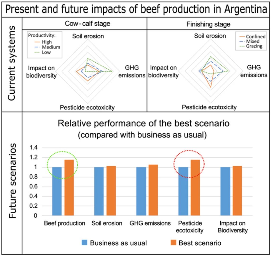
We analyse the current and future environmental impact of beef in Argentina, comparing four environmental dimensions (GHG, ecotoxicity, erosion and biodiversity) across 21 cow-calf systems and 47 finishing systems. The cow-calf and the finishing stages contributed equally to beef production, but impacts varied between stages (70 % of soil erosion and 75 % of GHG emissions occurred during the cow-calf stage, whereas 72 % of impact on biodiversity and 99 % of pesticide ecotoxicity occurred during the finishing stage). More intensive systems showed higher ecotoxicity and impact on biodiversity, and lower emissions and erosion per kg of beef than the more extensive systems. However, the intensity of this trade-off varied regionally, being more noticeable in the central regions of the Pampas and less so in the peripheric non-pampean regions. We also projected future beef production and environmental impacts under different production scenarios and found that it might be possible to increase beef production in Argentina by 15 % without a significant increase in the environmental impact of the sector (given a reduction of the ecotoxicological impact of crop production). We also showed that this could be achieved by adopting available practices and that the sector's self-set goals are compatible with this scenario.
The environmental impact of beef production has been the focus of a lot of research in the past decades (Eisler et al., 2014; Godfray et al., 2018; Herrero et al., 2015; Steinfeld et al., 2006). This interest was originally fuelled by concerns about methane emissions associated with enteric fermentation, that — together with deforestation to clear up land to produce feed — have positioned beef as one of the main anthropic sources of greenhouse gases (˜6 % of total human induced GHG emissions; Gerber et al., 2013). Concerns about the environmental impact of beef have led to many calls to reduce beef consumption and to change beef production systems (Springmann et al., 2018a). Despite all this, is likely beef production will continue to grow, and that growth needs to happen without increasing the environmental impact. When discussing beef sustainability, the extreme focus on GHG can be problematic (Röös et al., 2013), as many strategies to reduce GHG emissions are known to have negative consequences on other dimensions (Herrero et al., 2016). Thus, any assessment on the sustainability of beef needs to include more than one dimension (Rotz et al., 2019) and consider possible trade-offs between impacts (Röös et al., 2013).
Beef production systems are quite diverse worldwide, as they are the result of the combination of local environmental characteristics, culture, and economies (Seré and Steinfeld, 1996). Thus, trade-offs between impacts change across regions, so that it is necessary to assess the diversity of local systems and to propose solutions that are applicable to local contexts (Eisler et al., 2014). The proposals to increase beef sustainability come in a wide spectrum, from input-based high-tech solutions — like cultured meat (Post, 2012) and an ‘antimethanogenic vaccine’ (Iqbal et al., 2008) —to knowledge-based low-tech approaches — as breeding programmes (Wall et al., 2010) and rotational grazing (Gourlez de la Motte et al., 2018). Besides a vast diversity of systems, there is also a huge variation in the efficiency of production (Robinson et al., 2011) so that there might be a great potential to increase production by just adopting best practice and closing the productivity gap among producers (Gerber et al., 2013; Pacín and Oesterheld, 2015).
Argentina is one of the five largest beef producers in the world, accounting for almost 5 % of global beef production (USDA, 2018a). Argentina also has the second highest beef consumption per capita of the world, at ˜54 kg of beef per person per year, and >85 % of production is consumed domestically (USDA, 2018b). Argentine beef production experienced several changes in the past decades, as competition for land with grain and oil crops favoured the emergence of confined systems and relegated cattle away from the temperate central regions on the Pampas, towards peripheric non-pampean regions (Arelovich et al., 2011; Paruelo et al., 2006). In most of the non-pampean regions, beef production was mostly done by small scale and semi subsistence farmers, and now they coexist with large scale commercial farms (Mastrangelo et al., 2019). The environmental consequences of these land use changes have been the focus of several studies (Paruelo et al., 2006; Viglizzo et al., 2011). In particular, studies on the environmental footprint of beef production in Argentina focused on a single impact dimension (e.g., GHG emissions; MAyDS, 2017) or were limited to the local scale (a single farm, or a small region; Jacobo et al., 2006; Mastrangelo and Gavin, 2012; Modernel et al., 2018). However, comprehensive studies on the environmental impact of Argentine beef production that look at several dimensions at the country scale are lacking.
Beef production in Argentina remained fairly stable since the 1970s, with most years yielding between 2.5 and 2.8 million tonnes (SENASA, 2017). Currently, the sector is proposing two main strategies to increase production to keep up with local demand and increase exports: to increase national weaning rate, which currently averages 68 %, up to 75 % (the rate in similar countries of the region, like Uruguay and Brazil) and to increase carcass weight by 10 % (Argentine Association of Animal Production, 2018; MAyDS, 2017). However, the environmental implications of these proposals have yet to be analysed. In this article, we describe and compare the environmental impact of different beef production systems in Argentina under current conditions, and we evaluate the impact of the pathways proposed by the sector to increase productivity.
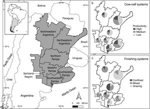
MethodsBeef production systemsThis study is based on a region of ˜1.24 million km2, which includes ˜45 % of the area of Argentina (Fig. 1a) and contains >90 % of the national herd (SENASA, 2017). The study area was divided in seven beef production regions, following MAyDS (2017): North-western Argentina (NWA, housing 9 % of the national herd), North-eastern Argentina (NEA, 27 %), Semiarid Region (SA, 6 %), Northern Pampa (NP,15 %), Western Pampa (WP, 11 %), South-eastern Pampa (SEP, 15 %) and South-western Pampa (SWP, 9 % Fig. 1). There is a clear difference in productivity between regions, considering that the average weaning rate in the central pampean regions is 73 % and drops to 66 % in the peripheric non-pampean regions (estimated from MAyDS, 2017). In addition, the average final weight in the pampean regions is 373 kg and is reached in 352 days, whereas in the non-pampean regions the average final weight is 393 kg and is reached in 497 days (estimated from MAyDS, 2017).
a) Map of the study area (in grey), showing the different beef production regions (MAyDS, 2017): North-western Argentina (NWA), North-eastern Argentina (NEA), Semiarid Region (SA), Northern Pampa (NP), Western Pampa (WP), South-eastern Pampa (SEP) and South-western Pampa (SWP). b and c) Distribution of cattle among the different production systems in each region for cow-calf (b) and finishing (c) stages. The size of the pie chart is proportional to the size of the herd in each region.
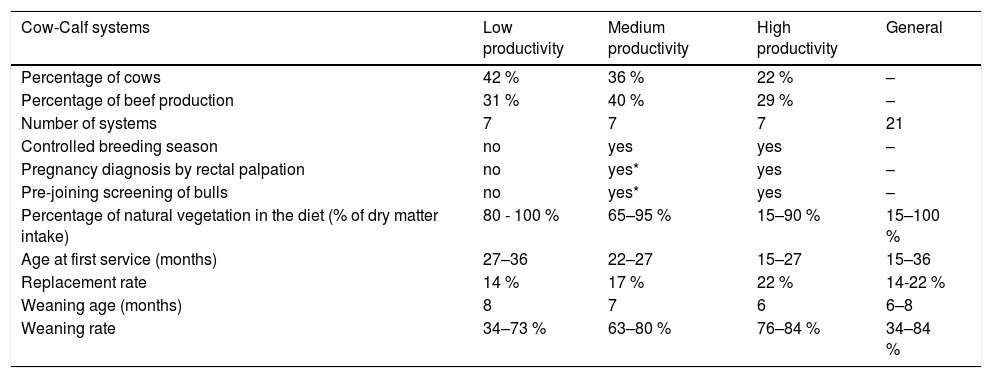
The beef production cycle in Argentina has two distinct stages: cow-calf and finishing. Cow-calf stage includes the reproduction process, producing calves of 165 kg live weight on average, which enter the finishing stage at weaning. Finishing stage can take many forms and sometimes it can be further divided in backgrounding and fattening. On average, the finishing stage produces steers/heifers of 383 kg after 425 days (MAyDS, 2017). To represent the diversity of beef production systems in the study area, the analysis followed the description of Modal Systems from the Second Biennial Update Report of the Greenhouse Gases Inventory of Argentina (MAyDS, 2017). All modal systems are defined first by the region they occur in. Then, cow-calf systems are characterized as low, medium and high productivity (one of each in each one of the seven regions, resulting in 21 systems in total), and differ among each other by diet composition, and reproductive and sanitary management, which resulted in a different characteristic weaning rate (see Table 1a, and Table I in the appendix for more details). All manure from cow-calf systems was assumed to be allowed to lie as deposited, without any management. Finishing systems in the study area are more diverse, with a total of 47 finishing systems, characterized by region, confinement, diet, length of finishing period, and final weight (MAyDS, 2017; see Table II in the appendix). For the purpose of this study, finishing systems were classified into three categories: grazing, confined and mixed (when animals spend a part of the stage confined and another part grazing; see Table 1b, and Table II in the appendix for more details). Each finishing system was assigned a specific manure management system, according to literature (MAyDS, 2017; see Table III in the appendix for more details).
There is a geographical variation in the distribution of cattle between systems. For cow-calf systems, low productivity systems tend to be more common in the northern regions (NWA, NEA, and NP). For finishing systems, intensification decreases radially from the centre of the study area — in the Pampas — with confined systems disappearing in NEA, SA, and SWP (Fig. 1b and c).
Herd modellingFor each cow-calf system, we modelled a herd with 100 cows during a whole cycle (from joining to weaning, see Figure I of the appendix) and estimated all the animal-days of each animal category involved, from the reproductive parameters of the system (described in MAyDS, 2017). As a whole cycle is longer than one year, it includes two reproductive seasons: one that will produce calves counted for this cycle and another that will produce calves that will be part of the next cycle.
First, we estimated the number of cows in each one of three pathways: 1) Lactating at first service and got pregnant in both services, 2) Lactating at first service and got pregnant in the first, but not the second service, and 3) Not lactating at the first service, but got pregnant in both services. The number of cows in pathways 2 and 3 was estimated from the replacement rate for the system, and the number of cows in pathway 1 was the difference between the total (100) and the two other pathways. Then, the number of animal-days for each category (lactating and gestating, not lactating and gestating, lactating and not gestating) was estimated for each pathway, in order to arrive to a total number of animal-days of each category for each system (see Figure I in the appendix). The number of replacement heifers was estimated from the replacement rate, and the days they were needed for, from the fattening length (MAyDS, 2017). The number of cows sent to slaughter was calculated from the replacement rate. The number of calves to be send to the finishing stage (Ni) was calculated as:
Where 100 is the number of cows in the modelled herd, Wri is the given weaning rate, and Rri is the replacement rate of the system i.Estimating beef productionFor cow-calf systems, we first calculated the amount of beef produced per calf, by multiplying the weaning weight by the carcass-weight to live-weight ratio for calves (0.55; MAyDS, 2017). Weaning weight for each region was calculated as the mean initial weight for finishing systems in the same region (see Table II in the appendix). The amount of beef produced per calf was then multiplied by the number of calves per cow in each system, in order to obtain the amount of beef produced per cow. We also calculated the amount of beef produced by culled cows. Then, the total amount of beef produced per year under each system was calculated by multiplying the amount of beef produced per cow by the number of cows present in each region (2016 stock; SENASA, 2017) and the proportion of animals in each system (see Figure II in the appendix; MAyDS, 2017).
For finishing systems, we calculated the amount of beef produced per steer/heifer, by multiplying the weight gain (final weight minus initial weight) by the carcass-weight to live-weight ratio for steers and heifers (0.56; MAyDS, 2017).Then, the total amount of beef produced under each system per year was calculated by multiplying the amount of beef produced per steer or heifer by the number of steers and heifers present in each region (2016 stock; SENASA, 2017) and the proportion of animals in each system (see Figure II in the appendix; MAyDS, 2017).
Estimating impactsThe intensity of the environmental impact of beef production in Argentina was calculated for four dimensions (soil erosion, GHG emissions, pesticide ecotoxicity and impact on biodiversity) for each production system in both stages, as described below (and see Figure III in the appendix for an overview). Impact intensity is expressed as impact per kg of beef (carcass weight) produced. Then, the absolute impact of each stage and of all beef production in the study area was calculated on the basis of the 2016 cattle stock per department (SENASA, 2017) and the distribution of cattle among the different systems in each region (MAyDS, 2017), by multiplying the values per kg of beef by the total amount of beef produced (see section 2.2).
Descriptions of agrochemical use in crops, and the estimation of erosion factors followed the regionalization of the 2017 edition of the Applied Agricultural Technology Survey (ReTAA, after its Spanish initials; Bolsa de Cereales, 2017). This survey divides the study area in 17 regions (ReTAA regions, see Figure IV in the appendix) that follow departmental divisions. Thus, each department in the study area was assigned to one beef region and one ReTAA region. For the impacts were ReTAA regions were used, the results are expressed by beef region, by combining the values of all departments in each beef region.
GHG emissionsDirect and indirect GHG emissions were estimated for each system, following a Tier 2 methodology (equations from IPCC, 2006; emission factors derived from data in MAyDS, 2017). We included CH4 emissions from enteric fermentation and manure management, as well as direct and indirect N2O emissions from manure management and from managed soils. First, we estimated the emissions per day for each animal category (lactating and gestating cows, not lactating and gestating cows, lactating and not gestating cows, steers and heifers) for each modal system, following the 2006 IPCC Guidelines for National Greenhouse Gas Inventories. In this calculation, the animal category defines the energy requirement of each animal, which is in turn used to calculate the total dry matter intake, and the digestibility of the diet of each system defines the emission factor per kg of dry matter. In turn, the diet (protein content) and animal category (N retention rate) determines the N excretion rate which, together with emission factors for different manure managing systems, were used for the calculations of N2O emissions. We used the number of animal/days of each animal category involved in the production of 1 kg of beef (calculated from the herd model, section 2.2.), and multiplied it by the emission factors of each category (lactating and gestating cows, not lactating and gestating cows, lactating and not gestating cows, and replacement heifers for cow-calf systems, and steer/heifers for finishing systems), to obtain a value of CH4 and N2O emissions per kg of beef. The results are presented in kg CO2 eq per kilogram of beef, using a 100 years Global Warming Potential for each gas (28 for CH4 and 265 for N2O).
Feed requirementAs the basis for the other impact estimations, we first calculated the amount of each feed item needed for producing one kilogram of beef in each system, as well as the land required to produce said item (see Figure III in the appendix). For cow-calf systems, all the reproductive herd (cows, bulls, and replacement heifers) was included. To this end, the number of animals of each category needed to produce one calf in each system — and the amount of time they are needed for — was calculated based on the reproductive parameters of each cow-calf system (Table 1a and see Table I in the appendix for more details). Then, the number of animals was divided by the weaning weight, to get the value per kilogram of beef produced. For finishing systems, the number of animals of each category needed to produce one kg of beef in each system — and the amount of time they are needed for — was calculated from the weight gain (final weight minus initial weight) and the length of the finishing period (see Table II in the appendix). The total amount of feed (dry matter) required for each system per kg of beef was calculated using the previous values and the energy requirements of each animal category, and the amount of each feed item was calculated from the diet composition for each modal system (MAyDS, 2017).
The area required to produce one kg of beef in each system was calculated by multiplying the amount of each feed item required and the amount of each item produced per hectare. For grazing, the data for dry matter production per hectare was provided with the description of the systems (MAyDS, 2017; see Table IV in the appendix). For crops (maize and sorghum), the average yield in each ReTAA region was used (Bolsa de Cereales, 2017).
Impact on biodiversityTo estimate the impact on biodiversity, we developed the Impact on Biodiversity Index (IBI).
IBI is formed by two components. The first one, Ai, is the area required to produce one kg of beef under system i (see section 2.4.2). This includes all the area required to produce the feed (grazed or harvested), and it is calculated from the diet description and the yield (for crops) or dry matter production per hectare (for grasslands and pastures) of each feed item. The result is expressed in hectares per kilogram of beef. The second component is based on the Agrobiodiversity component of the Grassland Conservation Index (developed by Parera and Carriquiry, 2014; and applied to beef production by Picasso et al., 2014), where pij is the proportion of the total area required to produce the amount of each feed item (i) required to produce one kg of beef under system j, and bj is the relative weight of each item (representing the difference in biodiversity from the natural vegetation). Thus, IBI is an expression of how much land is required to produce one kilogram of beef weighted by the relative impact of each land cover on biodiversity. For this calculation, all feed items were classified in four categories (each one with a particular coefficient bj), following the classification from Parera and Carriquiry (2014): natural vegetation (b = 1), perennial pastures (b = 0.9), annual pastures (b = 0.5), and crops (b = 0.4).Soil ErosionHydric soil erosion was calculated via the RUSLE equation (Renard et al., 1991):
where A is estimated average soil loss in tons per hectare per year, R is the rainfall-runoff erosivity factor (estimated from the mean annual rainfall in each ReTAA region, data from INTA, 2018), K is the soil erodibility factor (estimated from the proportion of each soil type in each ReTAA region, data from Cruzate et al., 2007), LS is the topographic factor (slope length and steepness, the same value was used for all regions; Gaitán et al., 2017), and C is the cover factor (for crops, the average of the most common rotations was used, and for grasslands and pastures a table value; Gaitán et al., 2017). Finally, a value per hectare of crop and grazing land for each ReTAA region was obtained, and the value for each system was calculated based on the area of each land use required to produce one kilogram of beef (all values used for this estimation can be found in Table V in the appendix). The result is expressed in kg of soil lost per kg of beef.Pesticide ecotoxicityThe ecotoxicity per kg of each agrochemical (herbicides, insecticides and fungicides) used was calculated with the USEtox 2.0 tool (Henderson et al., 2011; Rosenbaum et al., 2008). Then, a value for ecotoxicity per hectare vas calculated for each land use in each ReTAA region. The quantity of each chemical used in crops (maize and sorghum) was obtained for each region from the ReTAA report. Agrochemical use in grazing lands was provided by specialists from the National Institute of Agricultural Technology (INTA, J. Otondo and C. Borrajo, personal communication). For this analysis, grazing lands were classified in 5 categories: natural vegetation, spray-topped pastures, pastures, summer grazing crops, and winter grazing crops. Finally, the pesticide ecotoxicity per kilogram of beef in each system was calculated by multiplying the pesticide ecotoxicity value per hectare of each land use and the number of hectares of each land use necessary to produce one kg of beef (see Tables VI, VII, and VIII in the appendix, for a description of the data used in this estimation). The result is expressed as the potentially affected fraction of species (PAF) integrated over time and volume per unit mass of a chemical emitted (PAF m3 day kg−1; Rosenbaum et al., 2008).
Data analysisThe impact intensity in each dimension (soil erosion, GHG emissions, pesticide ecotoxicity and impact on biodiversity) between system types (high, medium and low productivity for cow-calf systems, and confined, grazing and mixed for finishing systems) was compared for each stage, via General Linear Models (Zuur et al., 2009), using ‘system type’ as the explanatory variable, ‘region’ as a blocking factor and each one of the impact dimensions (soil erosion, GHG emissions, pesticide ecotoxicity and impact on biodiversity) as the response variables. In the cases where the assumption of homogeneity of variance was not met, heteroscedasticity was modelled with the function Power of covariate (Zuur et al., 2009).
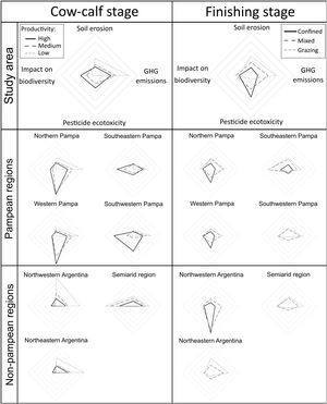
Possible trade-offs between impacts in different production systems for both stages, and their behaviour in different regions were explored via radar plots. All values are represented relatively to the maximum value for each impact dimension in each stage (which takes the maximum value). All graphs for one stage are presented in the same scale, as to allow direct comparison between regions, as well as system types (but not between stages).
ScenariosFor the cow-calf stage, we proposed two interventions in order to reduce the productivity gap among producers and thus simulate the proposed increase in weaning rate: 1) to redistribute all the cattle in the low productivity system of a certain region between the high and medium productivity systems in the same region (maintaining current proportions), and 2) to assign all cattle in each region to the higher productivity systems. Sub-scenarios (Bai et al., 2002) for cow-calf systems were created by simulating the application of each intervention, resulting in three sub-scenarios for this stage: Business as usual (BAU), Increased productivity and Maximum productivity (Figure V in the appendix).
For the finishing stage, we proposed two interventions to simulate an increase in final weight: 1) to transfer all the cattle in grazing systems to the grazing system with the higher final weight in the region, and 2) to simulate and increase in the length of confined systems in order to reach a 10 % increase in carcass weight (representing a 18 % increase in final live weight). The extension of the finishing period was calculated using a constant growth rate (Pordomingo, 2018). The sub-scenarios for the finishing stage were constructed by simulating the application of each one of the interventions, as well as the combination of both, resulting in four sub-scenarios for the finishing stage: BAU, longer confinement, heavier grazing, and both interventions (i.e., longer confinement + heavier grazing; Figure V in the appendix).
Finally, we created scenarios by assessing all combinations of sub-scenarios for both cow-calf and finishing stages (Figure V in the appendix). For each scenario, we calculated the changes in production and in each of the four impact dimensions in both relative and absolute terms. All sub-scenarios were created assuming no changes in the cattle stock in each region. However, for the combined scenarios, the stock entering the finishing stage reflected the increase caused by the corresponding cow-calf scenario, so that extra calves produced in each region were assigned to the finishing systems of the same region, following the same proportions observed in the business as usual scenarios.
Considering the many different data sources used, the multi-step calculations and multiple simplifications made in this analysis, we adopted as a decision rule that to say that either beef production or any of the impacts had changed, the difference between a certain scenario and business as usual had to be greater than |5|%.
ResultsThe amount of beef production in Argentina followed a similar geographic pattern than the distribution of cattle described previously (Section 2.1): 52 % of beef production comes from the pampean regions (15 % from NP, 15 % from SEP, 11 % from WP, and 11 % SWP), 32 % comes from NEA, 9 % from NWA and 7 % from SA. On the other hand, some regions specialize in one particular stage of beef production, with SEP specializing in the cow-calf stage (being responsible for 22 % of cow-calf beef production and 9 % of the finishing stage) and NP specializing in the finishing stage (11 % of beef of cow-calf systems and 20 % of beef from finishing systems).
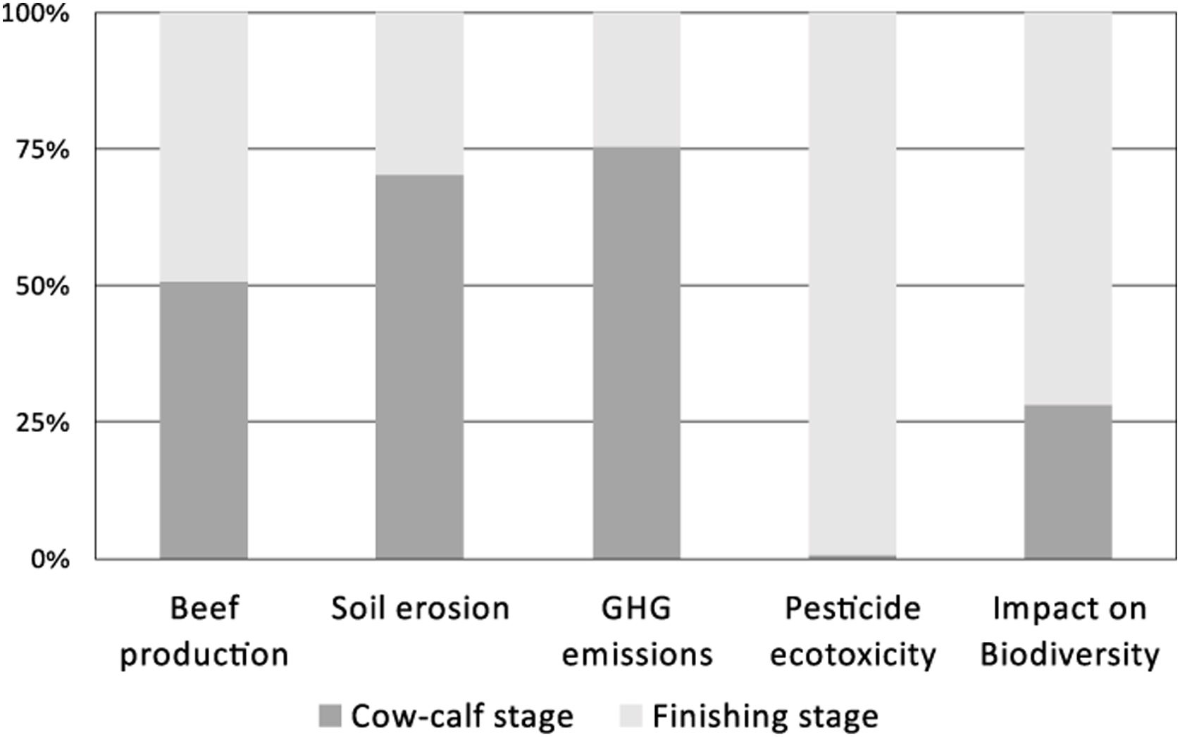
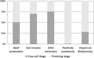
On average, cow-calf and finishing stage contributed about half of the slaughter weight each. However, impacts varied greatly according to production stage, so that most of the soil erosion and GHG emissions occurred during the cow-calf stage (70 % and 75 %, respectively) whereas most of the impact on biodiversity (72 %), as well as practically all the pesticide ecotoxicity (99 %) occurred during the finishing stage (Fig. 2).
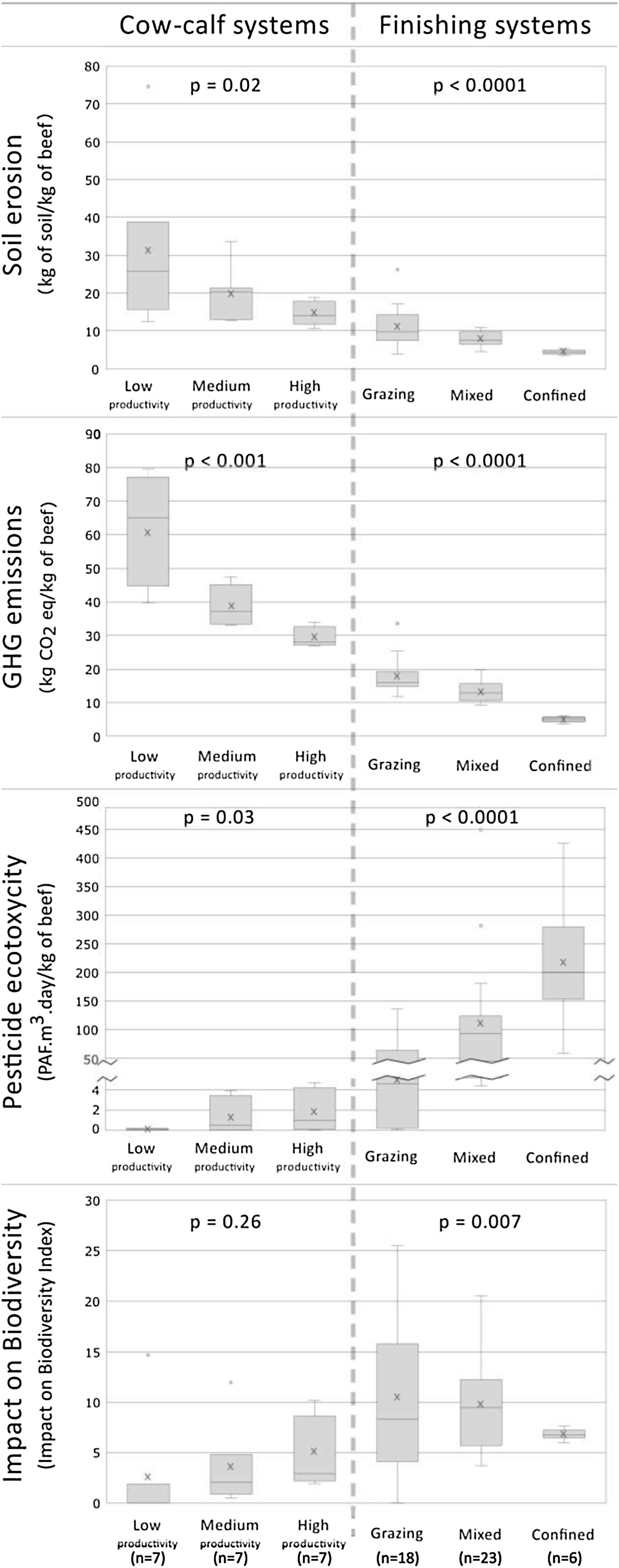
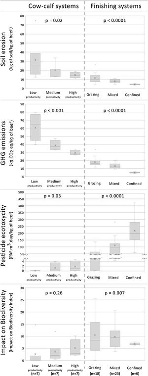
We found a trade-off between impacts, where high productivity cow-calf systems had lower soil erosion and GHG emissions and higher pesticide ecotoxicity per kg of beef than low productivity systems (p = 0.02, p < 0.0001 and p = 0.03, respectively; Fig. 3). Although we found no statistically significant difference in the impact on biodiversity between cow-calf systems (p = 0.26), data trends suggest it increases with productivity (Fig. 3). In addition, the trade-off was negligible in peripheric non-pampean regions (NWA, NEA and SA) compared with the central pampean regions (Fig. 4).
Impact intensity for different beef production systems in Argentina: low, medium, and high productivity cow- calf systems (left), and grazing, confined, and mixed finishing systems (right). Crosses mark the mean value, and boxes and whiskers indicate quartiles. Above each graph, p values for the GLM used to compare systems in each stage, are shown.
The finishing stage showed the same kind of trade-off between impacts as observed in the cow-calf stage: confined systems (the most intensive systems) presented lower soil erosion and GHG emissions, and higher pesticide ecotoxicity and impact on biodiversity than grazing systems (p < 0.0001 for soil erosion, GHG emissions and pesticide ecotoxicity and p = 0.007 for the impact on biodiversity; Fig. 3). No overall trend was noticed in the intensity of the trade-off between regions for the finishing stage (Fig. 4).
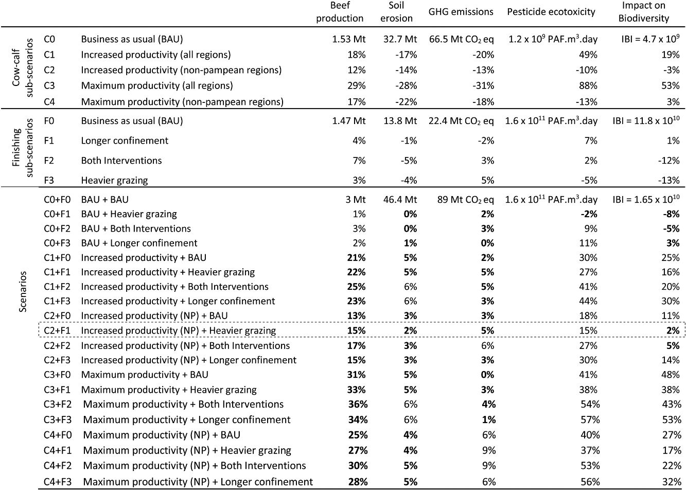
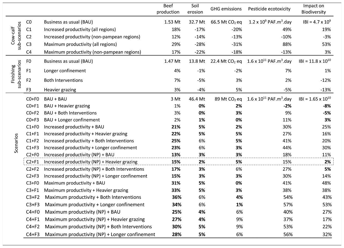
ScenariosThe proposed interventions rose average weaning rate in the study area from 70 % (estimated in the business as usual scenario) to 73–81 %, and average final weight went from 383 kg (in 425 days) to 390−398 kg (in 429–458 days, see Tables IX and X in the appendix). All interventions increased beef production, even though the changes to the cow-calf stage (i.e., increasing weaning rate by a switch towards systems with higher productivity) had stronger effect increasing beef production (12–29 %) than changes to the finishing stage (i.e., increasing final weight; 3–7 %; Table 2).
The two sub-scenarios for the cow-calf stage (“Increased productivity” and “Maximum productivity”) reduced soil erosion and GHG emissions but increased pesticide ecotoxicity and the impact on biodiversity (Table 2). Considering the different patterns observed in different regions (Fig. 4), we created two new cow-calf sub-scenarios where the interventions were only applied in the non-pampean regions (NWA, NEA and SA), where there was little or no trade-off between impacts. These new sub-scenarios increased production without increasing any impact (Table 2). For finishing systems, all sub-scenarios maintained most impacts at similar levels than the BAU scenario, but the increase in production was modest (up to 7 %, Table 2).
The combination of all sub-scenarios from both stages resulted in 20 scenarios for beef production in Argentina. All combined scenarios — except those based on BAU for the cow-calf stage — increased production (13–36 %). Most of them lowered soil erosion and GHG emissions per kg of beef, around half reduced the impact on biodiversity per kg of beef, and only one reduced the pesticide ecotoxicity intensity (see Table XI in the appendix). However, most scenarios increased all absolute impacts (Table 2). No scenario produced an increase in production without raising some of the absolute impacts. The best performance (i.e., increasing beef production while minimising the increase of its impacts) was from the scenario that combined “Increased productivity in the non-pampean regions” for the cow-calf stage with “Heavier grazing” for the finishing stage, where production increased by 15 %, and only pesticide ecotoxicity increased (by 15 %), while the other three impacts where kept at the same level as BAU scenario (Table 2).
DiscussionOur results show that the cow-calf and the finishing stages contributed equally to beef production in Argentina, but impacts varied between stages. More intensive production systems showed higher ecotoxicity and impact on biodiversity, and lower emissions and erosion per kg of beef than the more extensive systems. However, the intensity of this trade-off varied regionally, being more noticeable in the central regions of the Pampas and less so in the peripheric non-pampean regions. We also projected future beef production and environmental impacts under different production scenarios and found that it might be possible to increase beef production in Argentina by 15 % without a significant increase in the environmental impact of the sector (given a reduction of the ecotoxicological impact of crop production). We also showed that this could be achieved by adopting available practices and that the sector's self-set goals are compatible with this scenario.
On the variability of beef production systems in ArgentinaOur results show a great variability in the environmental impact of beef production systems in Argentina, where impact levels change according to the production stage, type of system, region, and impact dimension considered.
Dividing the analysis by stage allows us to plan mitigation strategies by identifying leverages and turning points. In Argentina, the cow-calf stage is responsible for most GHG emissions since this stage involves a larger number of animals (i.e., the reproductive herd), and each one of those animals contributes to GHG emissions, but they do not necessarily contribute directly to beef production. The great contribution of the reproductive herd to GHG emissions intensity has been noticed, and one of the usual mitigations strategies is to increase the efficiency of reproduction to reduce the burden of the reproductive herd (Gerber et al., 2013). On the other hand, our findings show that the finishing stage in Argentina accounts for most of the pesticide ecotoxicity and the impact on biodiversity, as crops present higher values for these impacts than grazing lands and crops represent a larger proportion of the diet in this stage. This also explains the fact that most of the soil erosion comes from the cow-calf stage: although grazing lands are associated with lower soil erosion per hectare than crops, larger extensions of land are required to produce the necessary feed, and thus the total soil erosion for cow-calf systems in Argentina is higher. It is worth noticing that cow-calf systems in other parts of the world can be much more intensive than in Argentina, with higher reproductive efficiency and more crops in the diet, and that would affect the relative contribution of each stage to each impact (Gerber et al., 2013; Robinson et al., 2011).
Our results regarding the trade-off between impacts are in agreement with studies pointing out that GHG emissions cannot be used as the sole indicator for the sustainability of beef production (Röös et al., 2013). The observed differences in the intensity of the trade-off between impacts for cow-calf systems from different regions can be explained by differences in base line productivity and input levels (MAyDS, 2017). In general, cow-calf systems in the central regions in the Pampas have higher productivity than those from the peripheric non-pampean regions (see section 2.1). In all regions, the increase in productivity for cow-calf systems is based in changes in reproductive and sanitary management and diet (Table 1). The improvements in reproductive and sanitary management are mostly the same in all regions, but diet changes are not: in the central pampean regions high productivity systems use more crops and grazing crops than in the peripheric regions (Table I in the appendix). As crops are associated with higher pesticide use, these changes in diet may cross a threshold and produce an increase in both pesticide ecotoxicity and impact on biodiversity. On the contrary, production in the peripheric non-pampean regions is less intensive (high productivity systems still rely mostly on pastures, instead of crops), so that there is room for further intensification without reaching that threshold. Mastrangelo and Gavin (2012) described a similar behaviour when looking at bird diversity along a cattle intensification gradient in North-western Argentina: intermediate-intensity silvopastoril systems yielded just 20 % less beef than high-intensity pasture systems, while maintaining ˜90 % of the bird species present in nearby forests (high-intensity systems maintained just ˜50 % of the bird species). The same applies to different parts of the world: at first, intensification increases productivity without a noticeable increase in environmental impact. However, pass a certain threshold (that would be different in each context and for each impact), any increase in productivity comes with a noticeable increase in environmental impact (Tscharntke et al., 2012).
Description of the different beef production systems in Argentina for cow-calf (a) and finishing (b) stages. Adapted from MAyDS (2017) *Except in Northern Pampa and Semiarid Region.
| Cow-Calf systems | Low productivity | Medium productivity | High productivity | General |
|---|---|---|---|---|
| Percentage of cows | 42 % | 36 % | 22 % | – |
| Percentage of beef production | 31 % | 40 % | 29 % | – |
| Number of systems | 7 | 7 | 7 | 21 |
| Controlled breeding season | no | yes | yes | – |
| Pregnancy diagnosis by rectal palpation | no | yes* | yes | – |
| Pre-joining screening of bulls | no | yes* | yes | – |
| Percentage of natural vegetation in the diet (% of dry matter intake) | 80 - 100 % | 65–95 % | 15–90 % | 15–100 % |
| Age at first service (months) | 27–36 | 22–27 | 15–27 | 15–36 |
| Replacement rate | 14 % | 17 % | 22 % | 14-22 % |
| Weaning age (months) | 8 | 7 | 6 | 6–8 |
| Weaning rate | 34–73 % | 63–80 % | 76–84 % | 34–84 % |
| b) Finishing systems | Grazing | Mixed | Confined | General |
| Percentage of steers/heifers | 42 % | 45 % | 13 % | – |
| Percentage of beef production | 45 % | 44 % | 11 % | – |
| Number of systems | 18 | 23 | 6 | 47 |
| Percentage of supplement in the diet (% of dry matter intake) | 8–55 % | 20–85 % | 100 % | 8 - 100 % |
| Initial live weight (kg) | 140–180 | 140–190 | 150–190 | 140–190 |
| Length of finishing stage (days) | 150–1080 | 180–720 | 150–270 | 150–1080 |
| Final live weight (kg) | 300–520 | 310–480 | 320–350 | 300–520 |
As a general rule, the larger the gap in efficiency between producers, the larger the potential to increase production with current technology, by just adopting best practice (Gerber et al., 2013; Pacín and Oesterheld, 2015). Available reports for Argentina show that the efficiency gap in cow-calf systems from the non-pampean regions (>100 %, Giancola et al., 2013), is larger than in the pampean regions (˜70 %, Némoz et al., 2013). The larger potential to increase production in non-pampean regions and the fact that there is further room for intensification (without increasing the environmental impact) in those regions, highlights non-pampean regions as the logical focus for the future development of the beef sector.
This study deals with lands that are currently under agricultural use and does not analyse the effects of the expansion of the agricultural frontier. However, it is important to keep in mind that the Chaco region (that overlaps in part with NWA and NEA in this study) is a global deforestation hotspot, and any further intensification processes have to rely on current agricultural land and/or be based in systems that maintain the forest cover. In this regard, this study only deals with current mainstream beef production systems, but there are many alternative beef production systems under development (e.g. Forests management with integrated livestock or MBGI), that might alter or eliminate the trade-offs between production and environmental impact and between different impacts.
On the analysis of scenarios for beef production in ArgentinaMany studies on beef sustainability focused just on impact intensity, and some authors have been reminding us that — as our results clearly show — impact intensity can be a useful metric when tweaking a production system, but proper scenario analysis needs to be based on absolute impacts (Garnett et al., 2015). Our results allowed us to detect one scenario that increases beef production in Argentina by ˜15 % without a significant increase in most of the absolute impacts, excepting for pesticide ecotoxicity which increased by 15 %. However, pesticide ecotoxicity impact could be reduced with changes in agrochemical use through integrated pest management (Abbas et al., 2018) and changes in crop selection (Coupe and Capel, 2016). Furthermore, improve grassland and pasture management could provide better quality feed for grazing systems, reducing the need to supplement diet with crops (Godde et al., 2018). For example, a study on the effect of rotational grazing in the South-eastern Pampa found and improvement in rangeland condition and in carrying capacity, achieving stocking rates 60 % higher than the average for the region (Jacobo et al., 2006).
Our results also clearly show that any significant change in beef production in Argentina requires interventions at the cow-calf stage, as all the scenarios that significantly increased beef production included some intervention at this stage (Table 2 ). On the other hand, changes in the finishing stage have the potential to moderate the increase in absolute impacts resulting from the increased production. The relative impact of interventions in each stage in both production and impacts might change across the globe (Pelletier et al., 2010).
Current absolute values for beef production and its environmental impacts in Argentina, and the percentage of change (relative to business as usual) under different scenarios. Values in bold are considered an improvement from BAU (for production, it means an increase >5 %, for impacts it means any decrease, or an increase ≤ 5 %). BAU = business as usual; NP = non-pampean region. Dotted line highlights the best performing scenario (i.e., the one that managed to increase beef production while minimising the increase of its impacts). See text (section 2.4) for a description of each scenario.
All scenarios considered in this study were based on practices that are currently available and have been proven to increase production and reduce — at least — some of the impacts, but the fact remains that not all producers have adopted them (Pacín and Oesterheld, 2015). Argentina has about 205 thousand beef farms, and a very high diversity in scale among beef producers: 52 % of beef farms have less than 100 cows and sum up ˜8 % of the national herd, whereas on the other hand 5 % of the farms have more than 1000 heads and concentrate ˜40 % of the national herd (SENASA, 2017). Furthermore, the structure of production varies greatly among regions. In Buenos Aires province (at the heart of the pampean region), 40 % of beef farms have less than 100 cows and sum up ˜5 % of cattle in the province and 8 % of the farms have more than 1000 heads and concentrate ˜51 % of the cattle. Meanwhile, in Chaco province (NWA) 84 % of beef farms have less than 100 cows and sum up ˜24 % of the cattle in the province and 1 % of the farms have more than 1000 heads and account for ˜34 % of the cattle (SENASA, 2017). Different producers face different barriers and need different solutions. In this regard, there are some local studies highlighting some possible barriers to the adoption of these practices in Argentina, and possible ways to overcome such barriers (Giancola et al., 2013; Némoz et al., 2013). Some of these barriers are due to a lack of knowledge, either about the existence of better practices or about when and how to apply them properly. For instance, producers still perform undiagnosed routine antiparasitic treatments, which could affect body condition and stimulate resistance. In these cases, extension services might help to increase adoption. In other cases, the barriers for adoption of best practices are economic: producers know how they could be more productive, but they lack the means or incentives to do it. For example, land tenure issues might deter producers from investing in infrastructure (paddocks, watering systems, etc.), and small-scale producers might not be able to cope with the fixed costs associated with more qualified workers or veterinarians. Legislation and public policies could help these situations by facilitating financing and regulating rental contracts. In this regard, Mastrangelo et al. (2019) analysed farm survey data from the Chaco region and found that the influence of access to credit and land tenure on gross revenue are higher for semi-subsistence than commercial farms, As semi-subsistence farms are more likely to have low productivity systems, both land tenure regularization and better access to credits have great potential to increase the productivity of the sector. Furthermore, in some cases barriers might be systemic, where professional or extension services, or infrastructure (e.g. electricity or roads) are missing. In these cases, it is necessary to improve rural infrastructure and extension networks. Finally, for some producers, livestock might not be their main activity. They do not have time or the inclination to allocate more resources to increase their productivity. In those cases, there might be ways to incentivise them to increase productivity, or to find alternative income sources.
ConclusionIn summary, our findings show that it is possible to increase beef production in Argentina around 15 % without a significant increase in the environmental impact of the sector. We also showed that this could be achieved by adopting best practice and that the sector's self-set goals are compatible with this scenario. Improvements in reproductive and sanitary management, as well as in diet quality could increase beef production in the non-pampean regions while maintaining the current environmental impact. However, this analysis is not a step by step guide towards the goal, but an exploration of a possible way forward and a demonstration of the potential of Argentine beef sector (with lessons to be learned for other countries; Eisler et al., 2014). We restricted the scenarios to what is achievable with practices and technology that are already applied in the region. Advances in breeding, pasture management and agrochemical use could lower the impacts even further in the future.
Although the particulars of this article apply mostly to Argentina, there are some generally applicable principles to derive from this analysis. First, sustainability is about more than just GHG or any single metric: GHG emissions are important, but they are not the only dimension we should be looking at. Second, there is a huge variety of beef production systems, and it is necessary to analyse each system on its own and to look at best practice and to focus on improving the efficiency of low performers, where a little change can generate a big difference. Third, it is important to evaluate absolute impacts of production, and not just their intensity (and to set goals in absolute terms). Finally, this study can contribute to the debate around “the beef issue”. Calls to reduce beef consumption come from both environmental and health related concerns (Springmann et al., 2018b). We do not address the health concerns here, but we believe this study adds to the debate over the environmental impact of beef by highlighting that not all beef is the same and production systems matters.
Declaration of interestsThe authors declare that they have no known competing financial interests or personal relationships that could have appeared to influence the work reported in this paper.
We would like to thank the National Directorate of Climate Change (Dirección Nacional de Cambio Climático, Ministerio de Ambiente y Desarrollo Sustentable de la Nación Argentina) for providing access to the beef section of the database for the National Inventory of Greenhouse Gases, and in particular, to the National Greenhouse Gas Inventory Team, for their help in explaining the GHG emissions calculations. We would also like to thank J. Otondo and C. Borrajo from INTA Chascomús, for their help describing agrochemical use in pastures, as well as the editor and two anonymous reviewers for their helpful comments on a previous version of this article. This research was financed by the University of Buenos Aires, Argentina (UBACYT 2017 - 20020160100010BA).
