Results from ecological niche models usually indicate a worrying scenario in terms of biodiversity loss. Continuous efforts to improve these models (e.g., allowing for dispersal limitation) have recently been updated to include the potential of species’ persistence, in otherwise unsuitable regions, due to natural selection (a process called evolutionary rescue). Here we discuss the major challenges in incorporating evolutionary rescue in models evaluating the impacts of global changes on species distributions. We also highlight some alternatives to overcome these challenges using simulations. Based on the current available evidence, we conclude that the potential of evolutionary rescue is low. However, due to the paucity of data to feed evolutionary rescue models and the interaction with other factors (e.g. habitat fragmentation), we still do not know the potential of adaptation to rescue biodiversity from climate change.
Biodiversity patterns are usually strongly correlated with climatic variation at different geographic scales (Hawkins et al., 2003). Based on the well-known effects of climate on species’ geographic ranges, it is possible to predict their responses under short-term climate changes, and this is the basis of the Ecological Niche Models (ENMs; see Peterson et al., 2011; Guisan et al., 2017). ENMs have been widely used tools for predicting geographic ranges shifts and considering the alarming rates of human-driven climate change (Garcia et al., 2014; Urban et al., 2016), a better understanding of these models and their correct application is critical to improve policies and guidelines for conservation and management (Araújo et al., 2019). The many problems with ENMs in predicting species’ response to climate change have been discussed elsewhere, but they can be summarized into two critical assumptions: equilibrium with current climate and niche conservatism (Holt, 2003; Araújo and Pearson, 2005; Hortal et al., 2012).
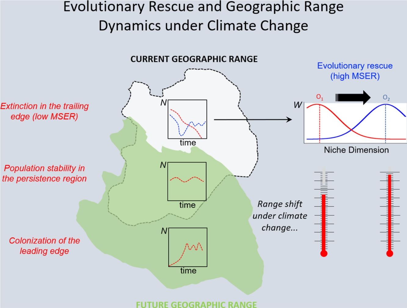
Under the two main theoretical assumptions of ENMs, we can recognize three regions within the species’ geographic range under the effects of climate change: (i) the persistence region, where future climatic conditions will remain similar to the current ones; (ii) the leading edge, where the future climatic conditions will become similar to the current ones, and; (iii) the trailing edge, a region where the climatic conditions will be very different from current conditions, so unsuitable for the species (see Ackerly, 2003; Diniz-Filho et al., 2019). We can then evaluate the dominant population-level processes in each of these three regions. In general, throughout the stable (or persistence) region, demographic rates will stay in equilibrium and thus there would be no significant trends in abundance, whereas long-range dispersal and population growth allowing colonization will be the main processes in the leading edge. Although ENMs usually assume unlimited dispersal ability (i.e., projecting species distribution throughout its leading edge) and despite the lack of reliable data on dispersal ability for most organisms, it is not difficult to explicitly incorporate dispersal in the modeling process (see Guisan et al., 2017). On the other hand, in the context of evolutionary rescue, it is important to focus on the species’ trailing edge, i.e., the future unsuitable region, which will be the focus of the reasoning developed below. This would be so because adaptation would be the main process that could avoid extinction of local populations inhabiting this region.
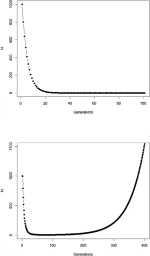
The new climate that will dominate in the trailing edge will, by definition, drive populations there to extinction because individuals are not well adapted to the new conditions. Simply stated, suppose that, before range shift, a population is in equilibrium so that its finite rate of increase λ is equal to 1. Assuming unsuitable conditions due to climate change (λ<1), a discrete model predicts a decline in population size toward extinction (Fig. 1A). However, this model assumes that all individuals within the population will be affected in the same way by the environmental change. On the other hand, in an evolutionary perspective, λ is the mean fitness of the population (Walsh and Lynch, 2018), given by ΣWi/N, where Wi is the number of offspring of the ith parent in the population with N individuals. But what if some of the individuals in the population are slightly better able to live in the new environment and thus will have more offspring than the mean λ? And what if this ability to live and better reproduce in the new environment is mediated by some inherited traits? This variation in fitness would occur due to the presence of individuals with pre-existing “resistance” to climate change and due to novel mutations (Bell, 2017).
Population trajectory of a simple discrete Malthusian model for a population starting with N0=1000 individuals. (A) Simulation with a fixed mean W=0.8 after an environmental change that reduces its mean fitness, goes to extinction after ca. 32 generations; (B) population trajectory if adaptive landscape in Fig. 2 increases mean fitness over time and allows evolutionary population rescue, with an h2=0.35 (see Gomulkiewicz and Holt, 1995 for details of this basic model).
The idea in the preceding paragraph is hardly new, being Darwin's breakthrough on natural selection (i.e., the Darwin–Wallace theory of natural selection, further mathematically elaborated by Pearson, Weldon, Fisher, Wright and Haldane, among many others, in the early 20th century). More formally, adaptation dynamics is summarized by a fitness function (Fig. 2) that will relate the individual fitness, W(z) with a trait z, so that
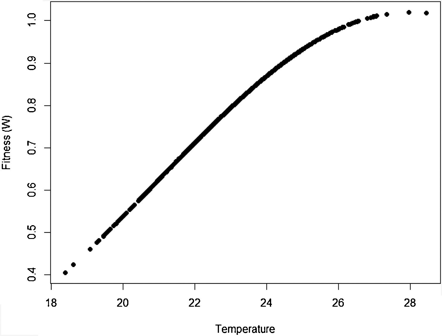
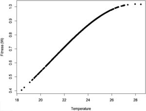
where Wmax is the fitness at the adaptive peak, or optimum value O for z, and w is the width of adaptive landscape. In the context of ecophysiological analyses related to climate change, the trait z can be one of the niche dimensions measured at the individual level, for example the body temperature (see Huey and Kingsolver, 1993). This Gaussian fitness function assumes stabilizing selection, and thus the distance of the mean phenotype from the optimum (in the new environment) at a time t, given by dt, will change aswhere σ2 is the total (phenotypic) variance of the trait z and h2 is its heritability, which is the proportion of the variance σ2 that is inherited. If h2 and σ2 are constant in time, the mean z will approach the optimum O following an exponential trajectory in time. The important consequence of this equation is that some individuals with, say, larger z-values will have a slightly large W, and if this z-value is inherited by their offspring according to h2, then a gradual shift in z and in the mean fitness will be observed. Also, this shift will result in a temporal dynamics of mean fitness W through time (t), according towhere E(W) is given by Wmax[w/(σ2+w)]1/2. Thus, better adapted individuals will gradually increase the frequency in the population and the mean fitness will go back to the original equilibrium value (λ=1). This is a simple mathematical formalization of Darwin's idea.Adaptive landscape, showing the relationship between fitness W and the target variable (here temperature), with optimum=28, w=100, so that at mean z=23 (the initial mean value of the population) the fitness is approximately 0.8. If no evolution occurs and mean fitness stays at W=0.8, the population will decrease as shown in Fig. 1.
In summary, although the population will decrease in the new environment, as predicted by the basic population growth model (because λ<1), this simple approach that we learn in basic population ecology courses ignores the role of natural selection. Then, population will persist if the time for the population to achieve zero (or a critical level) is longer than the time that natural selection will take to get the mean fitness back to 1. This is a direct consequence of the variance σ2, its inherited fraction (h2) and the strength of selection given by w. The equations shown above are the basis of the model proposed by Gomulkiewicz and Holt (1995) and can allow an easy understanding of what has been called “evolutionary rescue” (see Bell, 2013, 2017; Gonzalez et al., 2013; Carlson et al., 2014) (Fig. 1B).
The model by Burger and Lynch (1995), on the other hand, is a bit more complex as it assumes that the environment will shift gradually in time. The basic idea that can be derived from this model, for operational purposes, is to calculate the maximum sustainable evolutionary rate (MSER), i.e., the maximum rate of adaptation allowed by the genetic and demographic parameters of the population. Thus, if the predicted environmental or climate changes are larger than this MSER, then phenotypes will be not able to track such changes and evolutionary rescue is unlike (see Kopp and Matuszewski, 2014). The MSER is given by
where σA2 is the (additive) genetic variance (given by h2σ2), λ is the maximum rate of population increase in the adaptive optimum (called B in the original notation of Kopp and Matuszewski, 2014), VS is given by the sum of the length of the adaptive landscape (given here by w, but symbolized as w2 in Kopp and Matuszewski, 2014) and the environmental variance σe2. The value of MSER is expressed in units called Haldanes, which can be compared with expected or empirical rates of environmental changes (see Kopp and Matuszewski, 2014; Diniz-Filho et al., 2019 for details). But the logic underlying Burger and Lynch (1995) model is still to evaluate conditions at which λ>1, under a given rate of environmental changes.Of course, other processes will act at the same time on local populations, creating a more complex demographic and genetic dynamics. For example, population variance may be reduced due to selection (i.e., the Fisher's fundamental theorem of natural selection) and by stochastic processes (drift) in finite populations. Alternatively, other process may restore variance, including mutations (but usually at a very low rate, i.e., 10−4σ2), and dispersal from neighboring populations, in a metapopulation system (for example, Razgour et al., 2019 provided a recent analyses of potential for evolutionary and demographic rescue by combing ENMs and population genetics data). From a demographic point of view, density-dependent processes can also be easily incorporated into these models, although in a first (declining) phase of the evolutionary rescue no important effects will appear due to these processes (see Burger and Lynch, 1995).
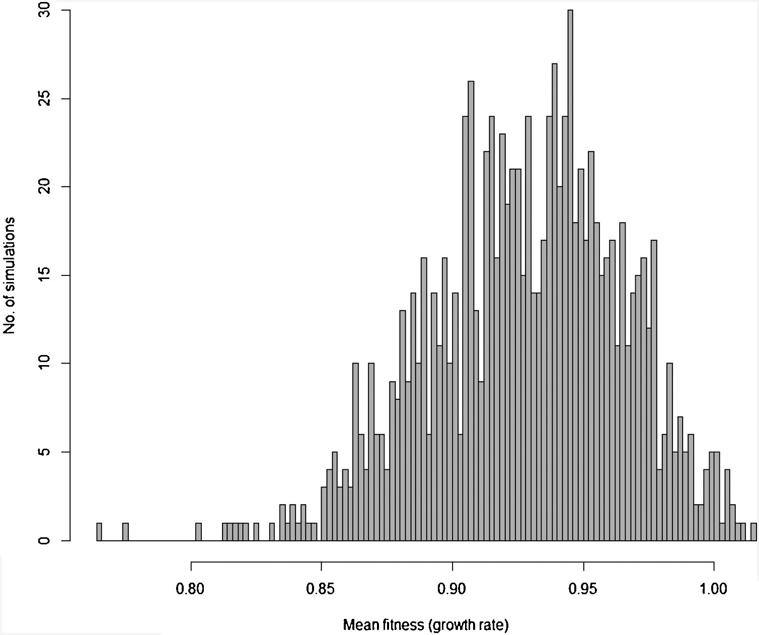
Moreover, besides adding stochastic effects and other processes driving population trajectory, it is important to consider that in most cases there are many uncertainties in defining the genetic and demographic parameters. These uncertainties can be incorporated in the more complex models using simulations allowing defining the probability of rescue given uncertainties due to processes and data (see Fig. 3 for an example). Finally, many traits will likely affect population fitness simultaneously. Thus, it would be advisable to work with multivariate models (although this will increase even more the number of parameters to be estimated, especially the total and genetic covariances among all these traits; see below).
Distribution of 1000 values for mean fitness of populations after 200 generations obtained by stochastic simulations based on Gomulkiewicz and Holt (1995) model, but incorporating loss and gain of genetic variance due to drift and new mutations, respectively, density-dependent population regulation (with K=N0=1000 individuals), and adaptive peak gradually shifting from 23 to 28 at each generation, as in Burger and Lynch (1995) model. Some of the parameters in each of the simulations based on this more complex model are also randomly sampled from uniform distributions, including the width of adaptive landscape w (ranging from 100 to 120), heritability h2 ranging from 0.3 to 0.4 and phenotypic variance ranging from 2 to 2.5. In this circumstance, different from the simple example in Fig. 1, the probability of evolutionary rescue (i.e., λ>1) after 200 generations is only 0.015.
Given that we can understand the processes described above, an important question is how plausible is evolutionary rescue under current anthropogenic climate change? Certainly, there has been a growing interest in this subject with different proposals for better integrating ecology and evolutionary biology to answer this question, which is one of the main questions in the “new” field that has been called “eco-evolutionary analyses” (Lavergne et al., 2010; Hoffmann and Sgrò, 2011; Norberg et al., 2012; Franks and Hoffmann, 2012; Thuiller et al., 2013; Hendry, 2017; Diamond, 2018). Indeed, adaptation has often been neglected as a mechanism involved in biological responses to climate change (Urban et al., 2016), inter alia, because the time scales have been considered too short to consider evolutionary processes. In practice, we still have a paucity of demographic and genetic data and, therefore, problems with model parameterization. Complex models are also quickly becoming available, especially those incorporating phenotypic plasticity (i.e., Chevin et al., 2010; Valladares et al., 2014). However, and again, they will require even more parameters that should be estimated in the field or with experiments for a large set of organisms.
One of the main difficulties when dealing directly with adaptation to climate change is the estimation of its variance of the variables related to species’ niche (as well as its genetic and plasticity components). This problem was recognized long ago in the context of ENMs, acknowledging that fundamental niches are larger than the realized and projected (by occurrence data) ones (see Peterson et al., 2011; Soberón and Arroyo-Peña, 2017 for a recent review and analysis). Ecologists and biogeographers have pursued the idea on how to add physiological experimental data within the ENM framework (see Kearney and Porter, 2009; see also Araújo et al., 2013). Results of these experiments would be of paramount importance to evolutionary rescue models because they would allow estimating the critical parameter σ2. However, the main problem with the ecophysiological experiments is that they usually estimate individual survival or mortality, whereas fitness (i.e., growth rate) is the parameter we need for evolutionary rescue models. It is also important to see how this fitness relates to critical traits to define the fitness function (Fig. 2), thus allowing to define w. These two parameters, σ2 and w, are critical for accurate predictions based on rescue models, and it may be challenging to estimate them for large-bodied and slow life-cycle organisms.
Thus, it is important to perform genetic experiments to estimate inheritance of traits related to climate change resistance, including the heritability and reaction norms in the parameters usually estimated in ecophysiological experiments. There are a few studies on this, although Diamond (2017) recently published a meta-analysis for Drosophila showing that heritabilities will tend to be low to moderate, which is expected considering our overall knowledge of heritability of physiological and life-history traits. Although the basic experimental design for estimating heritabilities and other genetic parameters is well established (see Lynch and Walsh, 1997), there are many challenges to perform new experiments for some organisms and natural populations. Recent molecular analyses of natural populations can provide a clue by associating phenotypic variation with genomic markers (Hendry, 2017). Until these problems are solved, we can use computer simulations to study the potential of evolutionary rescue with basis on a plausible range of parameters and to evaluate the robustness of conclusions under uncertainty. For example, Diniz-Filho et al. (2019) compared the projected climate change rates (expressed in Haldanes) for an amphibian species in Central Brazil with a statistical distribution of MSER generated by 5000 random combinations of several parameters sampled from plausible ranges (for example, h2 ranging from 0.2 to 0.4) and showed that the probability of rescue for shifts in the mean temperature is only 11% (see also Fig. 3 for a similar approach).
Quintero and Wiens (2013) showed that rates of niche evolution necessary to overcome the anthropogenic rates of climate change are much higher than macroevolutionary rates estimated using phylogenetic methods. However, these analyses are based on a gradualistic approach across deep time, so population analyses may be more realistic and account for rapid niche shifts and accelerated evolutionary rates under environmental stress. Unfortunately, most of the few empirical analyses found that rescue may be limited given the current rates of climate change (e.g., Lindsey et al., 2013; Urban et al., 2014; Alexander, 2013; Carlson et al., 2014). The potential of evolutionary rescues is likely to be strongly reduced if we consider interactions with other threats (e.g., habitat fragmentation), because they reduce dispersal rates and create strong population structure (reducing even more the critical parameter σ2). However, fast life-cycle organisms, including insects, annual plants and microorganisms, may provide some empirical examples of successful rescue. Ironically, this rescue may be problematic for our own species in terms of public health (see Hoffmann and Sgrò, 2011; Carlson et al., 2014; Bell, 2017). However, it is important to recognize that models incorporating plasticity provide more optimistic probabilities of persistence of populations, buffering extinction that may allow adaptation by further genetic canalization in some cases (e.g., Urban et al., 2014).
In a recent study, Cotto et al. (2017) showed that evolutionary adaptation is unlike to prevent the decrease in range of Alpine plant species predicted by ENMs. Moreover, they showed that reduction in fitness will happen before detectable range shifts occur, so demographic and genetic data of the local populations may be the first and more important early-warnings for threats. At broader geographic scales, there have been some attempts to incorporate evolutionary rescue and adaption in the context of ENMs (e.g., Bush et al., 2016; Diniz-Filho et al., 2019). By addressing the effects of phenotypic plasticity and the difficulties in estimating genetic variance of tolerances, Diniz-Filho et al. (2019) indicated that population persistence may be possible in some areas of the trailing edge. However, the main results of both studies cited above indicated a low potential of evolutionary rescue.
Thus, in conclusion, the short answer to the main question (“will life find a way out?”) we point out in this piece is: we simply don’t know…yet. Although models on evolutionary rescue may provide an integration of ecology and evolution to solve a practical and urgent problem for Humanity, we still do not have enough data to feed these models in a more realistic sense. The few empirical analyses based on appropriate data are not entirely conclusive about adaptive potential. Also, although species have faced large climate changes in the recent past (see Hof et al., 2011), current climate change also interacts with other anthropogenic threats. This complicates achieving a final idea on the impacts at higher hierarchical or aggregated levels (e.g., biodiversity and ecosystem functions). We hope that the ideas discussed above provide a longer answer that may be useful to improve models and data.
We thank two anonymous reviewers for suggestions that improved initial versions of this manuscript. This opinion piece resulted from a working group on “Evolutionary Rescue” promoted by our National Institutes for Science and Technology (INCT) in Ecology, Evolution and Biodiversity Conservation, supported by MCTIC/CNPq (proc. 465610/2014-5) and FAPEG (proc. 201810267000023). Works by J.A.F.D.-F. and L.M.B. are also supported by CNPq productivity fellowships. J.A.F. D.-F. is also supported by the Brazilian Research Network on Climate Change (CNPq No. 550022/2014 and FINEP No. 01.13.0353.00).

