

We aimed to evaluate the role of spatial units with different shapes and sizes on road-kill modeling for small vertebrate species. We used the road-kill records of two reptiles, water snake (Helicops infrataeniatus) and D’Orbigny's slider turtle (Trachemys dorbigni), and three mammals, white-eared opossum (Didelphis albiventris), coypu (Myocastor coypus) and Molina's Hog-nosed skunk (Conepatus chinga). Hierarchical partitioning was used to evaluate the independent influence of different land-use classes on road-kill by varying the shape and size of the spatial units. Variables that most explained road-kill were consistent over the different spatial unit types. The standard size seemed to be a reasonable solution for these species. Prior analysis with several sizes and shapes is needed to identify the appropriate spatial unit to model road-kill occurrence for larger vertebrates with different history traits.
In recent decades, researchers have used the available locations of wildlife–vehicle collisions (WVC) to model distribution patterns along roads and implement measures to minimize the road mortality rate (Gunson et al., 2010). Because different ecological patterns are created by processes occurring at different spatial scales (Collinge, 2001), the role of spatial units in characterizing the context of road–wildlife interactions is needed (Barrientos and Miranda, 2012). In general, a spatial unit comprises two different components: shape (point or road segment) and size (the area by which a point or road segment is buffered). Although the majority of mortality studies have mainly focused on spatial units of segments of 1000m/1 mile in length (e.g. Grilo et al., 2011), unit sizes are arbitrarily chosen, ranging from 50m to 5000m for the buffer radius (e.g. Barrientos and Bolonio, 2009; Colino-Rabanal et al., 2011) and from 100m to 1000m for the road segment length (e.g. Malo et al., 2004; Jancke and Giere, 2011).
The influence of the spatial unit shape and size in determining the factors that explain the likelihood of WVC is poorly known. Only a few studies have compared the unit size when using buffers to identify the features promoting road-kill with contrasting results (e.g. Colino-Rabanal et al., 2011; Danks and Porter, 2010). The wrong choice of spatial units may affect the identification of factors explaining WVC and therefore, the placement of mitigation measures will be biased and ineffective. Here, we argue that the selection of the spatial units is species-specific depending critically on their life-history traits.
The main goal of this study is to investigate whether changes in either the size of spatial units or their shape alter the road-kill risk. Using records of small vertebrates with different life-history traits, we evaluated whether variables related to the mortality risk vary according to the shape and size of spatial units. We also analyzed the variance explained by these variables among spatial units with different shapes and sizes.
In the absence of road- and landscape-related features at the microscale, we used land use data as predictors of habitat quality, which play a key role in road-kill models by improving their predictive capacity (Roger and Ramp, 2009). Because small-sized species and habitat specialists are more focused on particular features of land use, we expect that variables may not vary when changing the shape and size of the units. Likewise, we expect that explained variance decreases as the spatial units size increases.
MethodsStudy areaThe study site is located in the coastal plain in Southern Brazil (Fig. 1). This region is characterized by a coastal plain with a low and rectilinear relief dominated mainly by wetlands associated with fresh- and salt-water lakes (Tagliani, 2003). A total of 137km of two Brazilian Federal paved roads was surveyed: BR392 (33km) and BR471 (104km) (Fig. 1). BR392 and BR471 are 2-lane roads with an average daily traffic volume of 247 vehicles and an average speed of 80km/h (Bager, 2006).
Target species
We focus our analysis on five species representing different life-history traits. Water snake Helicops infrataeniatus is an aquatic species and is particularly vulnerable to road mortality (e.g. Bager and Fontoura, 2013). D’Orbigny's slider turtle Trachemys dorbigni is a fresh-water turtle with an observed road-kill rate of 0.23 individuals/100km/day (Bager and Fontoura, 2013). White-eared opossum Didelphis albiventris is a habitat generalist, solitary and omnivorous species with a high road-kill incidence (Cherem et al., 2007). Coypu Myocastor coypus is an aquatic rodent with a road-kill rate of 8.25 individuals/100km/day in BR471 (Bager and Fontoura, 2013). Molina's Hog-nosed skunk Conepatus chinga is a carnivore species that is widespread in southern Brazil (Cheid et al., 2006).
Data collectionRoad-kill dataRoad-kill data were obtained from URUBU System database (http://cbee.ufla.br/portal/sistema_urubu/). The locations were recorded weekly from January to December 2005 by car at approximately 50km/h, with at least two observers, avoiding weekends, holidays and rainy days. Road surveys (n=52) were performed between 7 am and 3 pm, and the road-kill locations were recorded with GPS.
Land-use dataWe used the land-use map from Tagliani (2003). We defined the following land-use classes: predominant rice field, sandbank vegetation, seaside fields, wetlands and non-native vegetation. Predominant rice fields are mainly covered by irrigated rice culture; sandbank vegetation are areas of low open arboreal vegetation that are influenced by the ocean and located high on dunes and slopes and on dry soil; seaside fields are flood fields of low grass; wetlands are floodplains with fertile clay soils; and non-native vegetation areas comprise eucalyptus and pine plantations (Eucalyptus sp. and Pinus sp.).
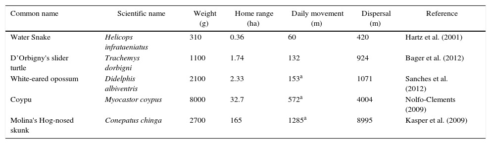
Definition of spatial unitsWe considered two shapes of spatial units: a buffer area around each road-kill location and road segments with a pre-defined length, where road-kills were assigned to each segment. We also considered three measures to define buffer diameters and road segment lengths: (1) the average daily movement length, (2) the standard size and (3) the average natal dispersal distance of each species (Table 1). The daily movement length was found in the literature or using information of the species average home-range size for mammals (see Bissonette and Adair, 2008). We used 1000m as the standard size used in several studies (e.g. Grilo et al., 2011). Because for water snake, no information on the home-range size was available, we used data from a study on a species of the same family (Liophis poecilogyrus) (Hartz et al., 2001). Natal dispersal information was found in the literature or estimated through Bissonette and Adair (2008) for mammals. For all of the spatial units, we extracted the area (m2) of each land-use class through ArcGIS 9.3 (ESRI, 2010).
Common and scientific name of species, the average weight and home-range size and the estimated daily movements length, and dispersal ability.
| Common name | Scientific name | Weight (g) | Home range (ha) | Daily movement (m) | Dispersal (m) | Reference |
|---|---|---|---|---|---|---|
| Water Snake | Helicops infrataeniatus | 310 | 0.36 | 60 | 420 | Hartz et al. (2001) |
| D’Orbigny's slider turtle | Trachemys dorbigni | 1100 | 1.74 | 132 | 924 | Bager et al. (2012) |
| White-eared opossum | Didelphis albiventris | 2100 | 2.33 | 153a | 1071 | Sanches et al. (2012) |
| Coypu | Myocastor coypus | 8000 | 32.7 | 572a | 4004 | Nolfo-Clements (2009) |
| Molina's Hog-nosed skunk | Conepatus chinga | 2700 | 165 | 1285a | 8995 | Kasper et al. (2009) |
Hierarchical partitioning (HP) was used to analyze the role of the shape and size of the spatial units in determining which land-use classes influence road-kill likelihood. This method identifies the key factors underlying the studied processes while reducing multicollinearity problems (Chevan and Sutherland, 1991). We determined the independent (I) contribution of each explanatory variable to the response variable and disentangled it from the joint (J) contribution resulting from correlation with other variables.
A sample of spatial units with an equal number of presence and absence of road-kill was used to estimate the percentage of model adjustment that was explained independently by each land-use class within all of the possible multiple regression models (Mac Nally, 2002). Buffers and segments with absence of road kills were randomly selected on the studied roads. We used the log-likelihood as a goodness-of-fit measure in HP. To assess the statistical significance of the variables, we followed the Mac Nally (2002) procedures. We ran 1000 randomizations of the data matrix to compute the distribution of the independent contribution of each predictor variable. The results were expressed with a significance of α=0.05 (Z-score>1.96). Hierarchical partitioning was performed using the “hier.part package” version 1.0 (Walsh and Mac Nally, 2004) from the R statistical software (R Development Core Team, 2006).
ResultsA total of 895 road-kills were recorded in the road surveys: 539 water snakes, 75 D’Orbigny's slider turtles, 76 white-eared opossum, 155 coypus and 50 Molina's Hog-nosed skunks. Thus, we obtained for the daily movement, standard and dispersal road buffer/segments the following number of samples with the presence and absence of road kill, respectively: 164, 67 and 98 for water snake; 108, 72 and 64 for D’Orbigny's slider turtle; 174, 110 and 114 for white-eared opossum; 68, 64 and 30 for coypu; and 64, 72 and 10 for Molina's Hog-nosed skunk.
Do variables related to the mortality risk vary according to the shape and size of the spatial units?We found consistency in determining the main variables explaining road-kill likelihood whether we used different shapes (buffer, segment) or unit sizes (Fig. 2). The variables that most explained the road-kills were seaside fields for water snake; predominant rice fields and seaside fields for D’Orbigny's slider turtle; sandbank vegetation and seaside fields for white-eared opossum; seaside fields for coypu; and predominant rice fields for Molina's Hog-nosed skunk (Fig. 2). Only one exception was identified for coypu: seaside fields showed a very low contribution (1%) to the road-kill occurrence at segment/dispersal compared to other shapes and sizes (variance explained ranged from 25% to 95%).
 1.96).' title='Percentage of variance in the occurrence of water snake (Helicops infrataeniatus), D’Orbigny's slider turtle (Trachemys dorbigni), white-eared opossum (Didelphis albiventris), coypu (Myocastor coypus) and Molina's Hog-nosed skunk (Conepatus chinga) road kills explained independently (I) by the five land-use variables for buffer and segment units. * – significant (α=0.05, Z-score>1.96).'/>
Percentage of variance in the occurrence of water snake (Helicops infrataeniatus), D’Orbigny's slider turtle (Trachemys dorbigni), white-eared opossum (Didelphis albiventris), coypu (Myocastor coypus) and Molina's Hog-nosed skunk (Conepatus chinga) road kills explained independently (I) by the five land-use variables for buffer and segment units. * – significant (α=0.05, Z-score>1.96).
Equally, we found no large differences in terms of the variance that was explained for the main variables regarding the shape and size of the spatial units (Fig. 2). However, we found more consistency in the variance that was explained for main variables when we used the buffer shape rather than the segment shape. We also observed that as the home-range size increased, the differences among the percentage of variance that was explained of the variables between shape and size also increased, except for in Molina's Hog-nosed skunk.
Interestingly, the variable that most explained the road-kill for the three species with smaller home-range sizes had a lower contribution at small spatial units than at larger spatial units. In contrast, smaller spatial units included variables with a higher contribution to explaining road-kill risk than larger spatial units for coypu and Molina's Hog-nosed skunk (species with larger home-range sizes). In general, the highest contribution of the most important variable in explaining mortality risk was expressed as the standard unit for species with small and large home ranges: 86% for water snake; 52% for D’Orbigny's slider turtle; 47% for opossum; 94% for coypu; and 53% for Molina's Hog-nosed skunk.
DiscussionAlthough the definition of the spatial units is complex and may be species-specific, our results show that the variables related to road-kills varied little with the shape and size of the spatial units and the most important variable explaining road-kill likelihood was, in general, consistent over different shapes and sizes for small vertebrates.
However, we found a few differences in the contribution of variables in the results. As hypothesized, species with larger home ranges showed less consistency in terms of variance that was explained by the main variables that were recorded at different shapes and sizes of spatial units. Likewise, the buffer shapes showed less dissimilarity among sizes than the segment shapes for species with higher home ranges. These species exploit a wide variety of habitats and food resources, being more able to explore distinct places according to resource supply (Basille et al., 2013). Interestingly, we found a higher contribution of the variables at larger spatial units for species with small home-range sizes and the opposite for species with larger home-range sizes, suggesting a good performance of the standard unit in this study.
The similarity of buffers compared to segments may be due to the location of the centroid of the spatial units. The buffer's centroid corresponds to the location of the road kill, and therefore, the buffer centroid keeps the same location at different sizes. The road segment's centroid does not correspond to the centroid of the road-kill because they are assigned to previously defined road segments. Thus, the road segments centroid varies as the segment length varies, leading to an expected variation in the results regarding the size of the spatial unit.
In agreement with other studies (Grilo et al., 2011), land-use variables that explain road-kill occurrence correspond to the preferential use of the vegetation structure of the five studied species. For example, Quintela et al. (2011) found a high use of seaside fields by water snake and coypu, corresponding to the variable that most explained road mortality in our study. Equally, white-eared opossum show a preference of low-density forest areas (Sanches et al., 2012), which corresponds to the sandbank vegetation structure (the most important variable in explaining road-kill). According to Bager et al. (2012), D’Orbigny's slider turtle is highly associated with temporarily flooded areas, and individuals are commonly found in drainage ditches in rice fields, which is the variable that most explained turtle road mortality. However, we found that some variables did not correspond to the suitable habitat for white-eared opossum and Molina's Hog-nosed skunk, as stated in the literature (Kasper et al., 2009).
The implementation of mitigation measures based on studies with the arbitrary use of spatial unit sizes and shapes is fragile. Our research highlights the importance of the spatial unit size and shape in analyzing road-kill data, considering species with different life history traits. Although the standard size seems to be a reasonable solution as it worked well for species with home range up to 165ha, our study underlines the importance of prior analysis with several sizes and shapes to identify the appropriate spatial unit for road-kill modeling for species with higher home-range sizes.
Conflicts of interestThe authors declare no conflicts of interest.
We are grateful for the various financial support provided by FAPEMIG (Process CRA – PPM-00139-14; 453 and CRA – APQ-03868-10), CNPq (Process 303509/2012-0), Fundação Grupo Boticário Process (0945-20122), and Tropical Forest Conservation Act – TFCA (through Fundo Brasileiro para Biodiversidade – FUNBIO). We thank the two anonymous reviewers for their constructive comments.

