


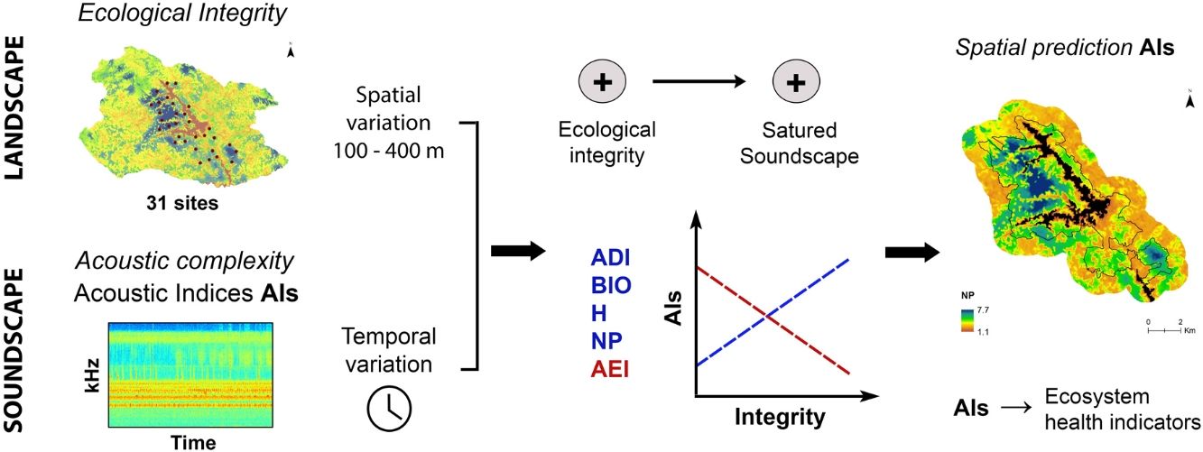
Soundscape research has acquired a paramount role in biodiversity conservation as it may provide timely and reliable information about the ecological integrity. The relationship between soundscape complexity and ecological integrity in highly biodiverse environments, as well as the factors affecting this relationship require a thorough understanding. We determined how the soundscape relates to the landscape ecological integrity at different spatial and temporal scales in a montane forest in the northern Andes of Colombia. Between May–July 2018 we obtained acoustic recordings from 31 sampling sites in the protected area of a hydropower plant, and estimated nine acoustic indices and an ecological integrity index (EII) derived from fragmentation, connectivity, and habitat quality. Five of the acoustic indices, linked to the evenness of the acoustic signals and levels of the biophonic signals, were associated with changes in the EII and indicated the presence of more even, saturated, and acoustically rich soundscapes in sites with higher integrity. Relationships between acoustic indices and the EII were stronger at a smaller spatial scale (100 m) and responded to daily variation of the soundscape, with the strongest associations occurring mainly from sunrise to noon. We show that acoustic indices measuring the evenness of the acoustic activity distribution and the number of frequency peaks reliably reflect the changes in the ecological integrity, and can be integrated with remote sensing as a tool for landscape management. Our results highlight the soundscape analysis as a feasible approach for the monitoring and conservation planning of acoustically unknown and threatened Andean landscapes.
Today’s world faces an evident biodiversity loss accelerated notably over the last half-century by growing anthropogenic pressures and ecosystem overexploitation (Dirzo et al., 2014; Jantz et al., 2015). Therefore, the need for fast and robust information to quantify the biodiversity state, and planning its conservation and management, is imminent (Pereira et al., 2013; Jetz et al., 2019). Current methods to monitoring biodiversity are usually expensive, requiring a great amount of time, resources, and expertise (Digby et al., 2013; Kallimanis et al., 2012). In the last decade, the use of environmental acoustic signals obtained through autonomous passive sensors has emerged as a cost-effective, non-invasive, and viable method for biodiversity assessment (Towsey et al., 2014; Sueur and Farina, 2015; Gibb et al., 2019). Through passive acoustic monitoring, simultaneous data collection from several sites across large areas allows a better understanding of the dynamics of acoustic communities and may provide reliable information about ecosystem health and habitat quality (Krause and Farina, 2016; Mammides et al., 2017; Zhao et al., 2019). However, this last role of acoustic signals is not well understood and yet need to be thoroughly examined before becomes a surrogate for ecosystem functioning (Farina, 2014).
Acoustic monitoring of all sounds emanating from an environment, or soundscape, begin to have an important role in biodiversity conservation, not only because the soundscape itself is a natural resource worthy for protection, but also because provide timely information about the health of landscapes and ecosystems (Dumyahn and Pijanowski, 2011; Farina et al., 2014). Acoustic signals within the soundscape include sounds from living organisms (biophony), natural sounds from physical processes (geophony), and sounds caused by human activities (anthrophony) (Pijanowski et al., 2011). These signals are related directly to the basic characteristics of the landscape (i.e., disturbance, species richness), and in turn, landscape elements (i.e., topography, vegetation patterns, animal distribution) are involved with the production and propagation of sounds (Farina, 2014; Farina and Fuller, 2017). This causal relation has led to the use of soundscape patterns as a rapid bioassessment tool at a variety of spatial and temporal scales, expecting to be a reflecting the ecological condition or integrity of a given area (Farina and Pieretti, 2012; Krause and Farina, 2016; Pavan, 2017).
The soundscape patterns are represented through acoustic diversity indices designed to estimate the heterogeneity of the sound regarding its time, frequency, and/or amplitude dimensions, and are considered as proxies of ecological complexity (Depraetere et al., 2012; Sueur et al., 2014). Previous soundscape studies assessing the relationship between acoustic patterns and ecological integrity have highlighted a consistent and positive connection of the integrity indicators with acoustic metrics indicating soundscapes acoustically rich, saturated, and with high levels of biophonic signal (Tucker et al., 2014; Fuller et al., 2015; Burivalova et al., 2018). These studies have considered integrity estimators based on components from site and landscape levels, including a variety of structural and functional attributes of vegetation, land-use type and intensity, patch size, and connectivity. Considering the ecological integrity as the ability of an area to maintain biodiversity and ecosystem processes (McGarigal et al., 2018), this positive connection is expected to be the consequence of a higher diversity of biophonic signals from more rich communities, and reflects the response of singing communities to changes in the condition or integrity of the habitat (Pijanowski et al., 2011; Servick, 2014).
Using the soundscape patterns as an integrity indicator requires a full comprehension of the influence of the factors intervening in the relationship on diverse environments. Previous studies have shown that different acoustic metrics are differentially connected to integrity indicators, and the relationship of some of them may exhibit patterns varying even between similar ecosystems (Fuller et al., 2015; Ng et al., 2018; Dröge et al., 2021). In addition, factors linked to landscape spatial variation, and the intrinsic temporal variation of the soundscape also could influence the relationship, as it has been documented in connections with other landscape elements (Mullet, 2017). Recent studies indicate that acoustic metrics respond to different spatial scales, with the magnitude of their associations with landscape elements being affected by how the scale delimiting the soundscape is defined and in which such attributes are estimated (Dooley and Brown, 2020; Dein and Rüdisser, 2020). Likewise, the connection between acoustic metrics and landscape elements may respond to the temporal dynamics of the soundscape, varying in magnitude across seasons or even emerging only at specific daily periods (Gage and Axel, 2014; Mullet et al., 2016).
In Tropical ecosystems, containing a more complex acoustic diversity and where acoustic monitoring has shown a great potential for animal richness and habitat assessment (Rodriguez et al., 2014; Campos-Cerqueira et al., 2020; Do Nascimento et al., 2020), the use of the soundscape patterns as an integrity indicator could be a useful tool for landscape monitoring. However, tropical soundscapes are largely understudied and the behavior of their relationship with the landscape elements yet needs thorough examination (Scarpelli et al., 2020). In this study, we investigate the relationship between soundscape complexity and the ecological integrity in a montane forest in the northern Andes of Colombia. To do so, we implemented an integrity index based on fragmentation, connectivity, and habitat quality indicators, and analyzed how nine acoustic indices relate to changes in the landscape ecological integrity at different spatial scales. Additionally, we assessed the influence of daily variation of the soundscape on these relationships. Given that soundscape can provide suitable information on the ecological condition or integrity of an area, we expect that greater soundscape complexity, represented by higher biophonic activity level, use of frequency bands, and evenness of acoustic activity distribution, will be related to greater ecological integrity. We show here how the soundscape patterns may reflect the ecological integrity and the potential of the soundscape analysis as a novel approach to the biodiversity monitoring and conservation planning of the Andean landscape.
Materials and methodsStudy areaWe studied the soundscape of a montane forest located in the eastern flank of the northern Cordillera Central in the Magdalena ecoregion in Colombia (Fig. 1). The area is a natural reserve comprising ca 50 km2, including the San Lorenzo reservoir (10.2 km2), dominated by different successional stages of forest (70% of the study area) and ranging from 1000 to 1400 m a.s.l. (Fig. 1). The region receives between 2000 and 4000 mm of annual precipitation and exhibits a bimodal rainfall regime with rainy seasons on March–May and September–November (Poveda et al., 2005). This area is considered a paramount site for biodiversity conservation at a regional scale as it maintains highly diverse communities of terrestrial vertebrates and plants, including threatened and endemic species (Restrepo et al., 2017; Sánchez-Giraldo and Daza, 2017).
 and land covers around the protected area of Jaguas Hydroelectric Power plant. Circles around sampling site represent the 100 to 400 m buffer areas used for the estimation of the ecological integrity index (EII).")
Study area in northern Cordillera Central, Colombia. Spatial distribution of 31 sampling sites (Table A1) and land covers around the protected area of Jaguas Hydroelectric Power plant. Circles around sampling site represent the 100 to 400 m buffer areas used for the estimation of the ecological integrity index (EII).
We obtained audio recordings from 31 sampling sites between May and July 2018. This period time covered the transition season when light-moderate intensity rainfalls can occur frequently, and in which a high acoustic activity has been documented for some vocalizing groups in the study area. Sites were located within the protected area and randomly selected considering forest (23 sites) and non-forest (eight sites) covers as strata, and using a proportional allocation according to the extension of each cover (Fig. 1, Table A1). We used a minimum distance of 800 m between sites to ensure spatial independence avoiding the overlapping of acoustic signals. On each sampling site, we deployed an autonomous recorder equipped with two omni-directional microphones (SongMeter SM4; Wildlife Acoustics, Inc.). The device was attached to trees at a height of 1.5 m above ground and programmed to continuously collect 1-min recordings every 15-min, using a sampling rate of 44.1 kHz, at 16 bits. The acoustic survey was carried out in groups of five sites, deploying a recorder during 5.0 to 9.6 consecutive days at each site. This data collection scheme resulted in 20,068 1-min recordings from all sampled sites (326–741 recordings per site) (Table A1).
Soundscape metricsWe selected nine acoustic indices to describe the acoustic heterogeneity of the soundscape in each sampling site (Fig. 2). Selected indices are categorized as complexity indices, which are based on the assumption that the complexity of acoustic output is proportional to a greater number of singing individuals and species (Sueur et al., 2014). Acoustic indices were estimated for each 1-min recording, applying an upper limit of 12 kHz in most of them. We chose this frequency limit to primarily analyze the acoustic complexity linked to the biophonic component, by assuming that most of the animal acoustic activity in our system is concentrated below 12 kHz (Sánchez-Giraldo et al., 2020). All indices were estimated using the default settings with the packages seewave v.2.1.4 and soundecology v.1.3.3 (Sueur et al., 2008a; Villanueva-Rivera and Pijanowski, 2016) in R v.3.6.1 statistical environment (R Core Team, 2019) (Table A2). Recordings containing rainfall sounds (3104 recordings) were not included for the calculation of ADI, AEI, BIO, H, M, and NDSI as they may affect indices values and the downstream analyses (Appendix B, Table A1).
 and documented soundscape patterns.")
Description of the acoustic indices used in this study, properties of the acoustic signals on which each index measure complexity, and soundscape patterns linked to high or low index values. Lines indicate the parameters of the property used in the estimation of each index. References correspond to the original description of each index (bold) and documented soundscape patterns.
We adopted a modified version of the framework proposed by Lee and Abdullah (2019) to measure ecological integrity, using as indicators the forest fragmentation, connectivity, and habitat quality, which have provided reliable integrity measurements in terrestrial landscapes (Reza and Abdullah, 2011; McGarigal et al., 2018). Maps for each indicator were generated on a focal area of 249.5 km2 (Fig. C1). We used as fragmentation indicator the Foreground Area Density (FAD) with forest cover being assigned as foreground (Riitters and Wickham, 2012) (Appendix D). FAD ranges between 0 to 100, with higher values indicating the presence and compactness of forest cover, and lower values corresponding to lower presence and higher fragmentation (Riitters and Wickham, 2012). Vegetation covers map of the focal area was based on the supervised classification of SENTINEL-2 images (September 2017, https://scihub.copernicus.eu/dhus/) (Appendix D).
Habitat connectivity was modeled from a perspective of terrestrial fauna requirements and the resistance to its movement due to the human impacts (Correa Ayram et al., 2017). We applied a circuit theory approach on a resistance surface based on a map of spatial human footprint index (SHFI) to generate a cumulative current flow map (McRae and Beier, 2007; McRae et al., 2008; Correa Ayram et al., 2017) (Appendix E). Circuit theory models the animal movement across a surface using the analogous relationship between the properties of random walk and electric current flow through a circuit (Doyle and Snell, 1984). To model connectivity in all directions, and generate an omnidirectional and unbiased current density map, we followed the method of Koen et al. (2014) and used random focal nodes on the perimeter of a buffer zone (see details in Appendix E). The cumulative current map obtained from combination of all pairwise connections is a prediction of functional connectivity, in which a high current flow in a pixel represents a high probability of use by random walkers (Koen et al., 2019).
To model habitat quality, we implemented a general approach in which an overall score was assigned to each quality proxy, according to their suitability for terrestrial vertebrate species associated with mainly forest areas, using non-volant mammals and anurans as focal groups (Appendix F). We calculated a cumulative indicator using as quality proxies the vegetation cover, transformed normalized difference vegetation index (TNDVI), bare soil percentage, percentage of photosynthetically active vegetation (PAV), terrain roughness, distance to water bodies, and distance to drainages. The final habitat quality map was obtained through the sum of the reclassified variables and the subsequent rescaling between 0 (lowest quality) and 100 (highest) (Appendix F).
From rescaled rasters (30 × 30 m spatial resolution) of fragmentation (FAD), connectivity (CON), and habitat quality (HQ) indicators, the ecological integrity index (EII) for each pixel was estimated as: EII = (FAD + CON + HQ)/Σ (FADmax + CONmax + HQmax); where FADmax, CONmax, and HQmax correspond to the maximum value of each indicator within the focal area. The EII ranges between 0 and 1, with values close to 1 indicating higher ecological integrity. We calculated the mean value of EII for each sampling site in four spatial scales, considering areas defined by 100, 200, 300, and 400 m radii buffer centered at the recorder installation point.
Data analysesWe analyzed the relationship between the acoustic indices and the ecological integrity of the landscape using generalized linear mixed-effects models (GLMER). We fitted models with acoustic indices values as the response variable, the ecological integrity index (EII) and hour of the day as independent fixed effects, and sites as a random effect. Models included an autoregressive covariance structure (corAR1) for the time (hour of the day) to account for potential temporal autocorrelation. To identify the scale at which acoustic indices are closely related to the ecological integrity, we built independent models for the EII estimated at each spatial scale. Likewise, we assessed whether the daily temporal variation of the acoustic indices affects their relationship with the EII. For this, we fitted models to each hour separately with the EII at spatial scale selected in the previous step as fixed effect and sites as a random effect. We fitted reduced models to assess the significance of random effect and the covariance structure (Table G1).
We built all models and checked for assumptions of mixed-effects models using the R packages glmmTMB (Brooks et al., 2017) and DHARMa (Hartig, 2019) respectively. The EII, estimated at all spatial scales, was standardized for improving model convergence. We fitted AEI, H, M, and NDSI values with beta error structure; ACI with gamma structure and log link function; ADI with Gaussian structure and log link function; NP with Poisson structure and logit link. BI and BIO values were normally distributed. Before the analyses, NDSI was transformed according to the formula (NDSI + 1)/2 (Fairbrass et al., 2017). We selected the best models based on the Akaike Information Criterion (AIC) (Akaike, 1973), and used as additional selection criteria of the spatial scale the highest value of the estimated coefficient and significance level (p-value <0.05) to the EII effect.
ResultsAcoustic indices showed high variation within sampling sites, with ACI, H, and NDSI exhibiting the lesser variation rates among indices (Table G1). Visual examination of acoustic indices indicated no trends in their spatial distribution in the protected area. Mean values from sampling sites did not show a pattern following sections within the area or linked to the distribution of vegetation covers or reservoirs (Fig. G1). Among indices, ADI, NDSI, and H had homogeneous and dominated by high values distributions (above 60–70% sampling sites) (Fig. G1). M exhibited a similar trend, but with mean values being low (<0.06) in the most of sites (68%). For the other indices, 45%–61% of sampling sites were dominated by medium values. In contrast to acoustic indices, the EII showed a spatial trend characterized by the concentration of highest values (EII > 0.75) in sites placed in deeper areas of forest cover, and lowest values in those around reservoirs and hydroelectric infrastructure (Fig. G2).
Among the nine analyzed acoustics indices, five (ADI, AEI, BIO, H, and NP) resulted in significant relationship with the ecological integrity (EII) (Tables 1, H1). Higher integrity values were strongly associated with higher values of ADI, BIO, H, and NP, and with lower values of AEI (Fig. 3A). These relationships were significant in all spatial scales, but models including ecological integrity estimated at 100 m were selected over the other scales (Tables H1, H2). Associations between the EII and BI, M, and, NDSI were not significant at any spatial scales. All models were best fit with a covariance structure and random effects, showing in all cases correlations above 0.80 and supporting the use of the autoregressive structure (Table H1). According to models at 100 m scale, AEI and NP had the largest changes in their values with the variation of the ecological integrity, reaching an estimated decrease and increase of 13.4% and 12.1% respectively relative to a 0.1 increase in the EII. This increase in the EII was associated with an increase of 5.5% on ADI, and 4.1% on BIO and H values (Fig. 3A).
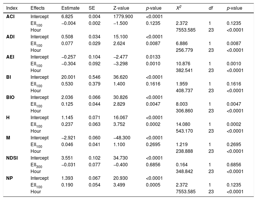
Mixed-effects models describing the relationship between acoustic indices and the ecological integrity index (EII) and hour of the day (Hour). Subscripts 100 and 300 indicate the spatial scale for the EII. Estimates of fixed effects and standard errors from conditional model, and their significance are indicated for EII and intercept. Overall significance for EII and Hour terms is indicated reporting X2, df, and P-value. Acoustic complexity index (ACI), Acoustic diversity index (ADI), Acoustic evenness index (AEI), Bioacoustic index (BI), Energy level of Biophony (BIO), Acoustic entropy index (H), Median of amplitude envelope (M), Normalized difference soundscape index (NDSI), and Number of peaks (NP).
| Index | Effects | Estimate | SE | Z-value | p-value | X2 | df | p-value |
|---|---|---|---|---|---|---|---|---|
| ACI | Intercept | 6.825 | 0.004 | 1779.900 | <0.0001 | |||
| EII100 | −0.004 | 0.002 | −1.500 | 0.1235 | 2.372 | 1 | 0.1235 | |
| Hour | 7553.585 | 23 | <0.0001 | |||||
| ADI | Intercept | 0.508 | 0.034 | 15.100 | <0.0001 | |||
| EII100 | 0.077 | 0.029 | 2.624 | 0.0087 | 6.886 | 1 | 0.0087 | |
| Hour | 256.779 | 23 | <0.0001 | |||||
| AEI | Intercept | −0.257 | 0.104 | −2.477 | 0.0133 | |||
| EII100 | −0.304 | 0.092 | −3.298 | 0.0010 | 10.876 | 1 | 0.0010 | |
| Hour | 382.541 | 23 | <0.0001 | |||||
| BI | Intercept | 20.001 | 0.546 | 36.620 | <0.0001 | |||
| EII100 | 0.530 | 0.379 | 1.400 | 0.1616 | 1.959 | 1 | 0.1616 | |
| Hour | 408.737 | 23 | <0.0001 | |||||
| BIO | Intercept | 2.036 | 0.066 | 30.826 | <0.0001 | |||
| EII100 | 0.125 | 0.044 | 2.829 | 0.0047 | 8.003 | 1 | 0.0047 | |
| Hour | 306.860 | 23 | <0.0001 | |||||
| H | Intercept | 1.145 | 0.071 | 16.067 | <0.0001 | |||
| EII100 | 0.237 | 0.063 | 3.752 | 0.0002 | 14.080 | 1 | 0.0002 | |
| Hour | 543.170 | 23 | <0.0001 | |||||
| M | Intercept | −2.921 | 0.060 | −48.300 | <0.0001 | |||
| EII100 | 0.046 | 0.041 | 1.100 | 0.2695 | 1.219 | 1 | 0.2695 | |
| Hour | 238.888 | 23 | <0.0001 | |||||
| NDSI | Intercept | 3.551 | 0.102 | 34.730 | <0.0001 | |||
| EII300 | −0.031 | 0.077 | −0.400 | 0.6856 | 0.164 | 1 | 0.6856 | |
| Hour | 348.842 | 23 | <0.0001 | |||||
| NP | Intercept | 1.393 | 0.067 | 20.930 | <0.0001 | |||
| EII100 | 0.190 | 0.054 | 3.499 | 0.0005 | 2.372 | 1 | 0.1235 | |
| Hour | 7553.585 | 23 | <0.0001 |
. Predicted values are estimated from fixed effects of conditional models (see Table 1). The shaded area indicates the 0.95 confidence interval. B. Temporal patterns of acoustic indices according time of day. Index values for each hour are predicted from fixed effect of conditional models (see Table 1). Dots and bars indicate the estimated mean and 0.95 confidence intervals respectively. Abbreviations of acoustic indices as in Table 1.")
A. Relationship between acoustic indices and the ecological integrity index (EII). Predicted values are estimated from fixed effects of conditional models (see Table 1). The shaded area indicates the 0.95 confidence interval. B. Temporal patterns of acoustic indices according time of day. Index values for each hour are predicted from fixed effect of conditional models (see Table 1). Dots and bars indicate the estimated mean and 0.95 confidence intervals respectively. Abbreviations of acoustic indices as in Table 1.
All acoustic indices varied significantly along the day, exhibiting differential diel patterns characterized by maximum values at diurnal (08:00−17:00 h) or nocturnal (20:00−05:00) times, or distinctive peaks at dawn (05:00−08:00) or dusk (17:00−20:00) periods (Table 1, Fig. 3B). BI, BIO, and M exhibited maximum values in different periods of diurnal time, and lower ones at dawn (Figs. 3B, G1). ADI and H showed a similar behavior than the previous indices, but higher values also included part of dusk period (19:00 h). Conversely, AEI and NP had higher values at nocturnal time and peaks at dawn and dusk periods respectively, and decreasing at morning hours (08:00−11:00 h). ACI exhibited maximum peaks at dawn and dusk periods, and NDSI had a peak decrease at 05:00−08:00 h and remained steady throughout the rest of the day (Figs. 3B, H1).
We found positive associations of the ecological integrity with ADI, BIO, H, and NP, and a negative correlation with AEI at specific hour of day. However, the observed variation of acoustic index values along the day was also reflected in the magnitude and significance of these relationships (Fig. 4). For instance, the EII was significantly associated with H at all hours, and with AEI and NP in almost all ones; while significant associations with ADI and BIO were concentrated in daylight hours. Regarding ACI, BI, and M, in which the relationships with the EII were not significant using complete time data, significant associations for some hours were identified. BI and M were positively associated with the EII between 15:00 and 17:00 h. ACI was the only index exhibiting significant associations in both directions: negative at late night and dawn and positive at 19:00 h (Fig. 4). In the case of NDSI, all hourly associations were not significant. We found that the relationship between the ecological integrity and acoustic indices was strongest in four periods of the day: at 06:00−8:00 h for BIO, H, and NP; 10:00−12:00 h for ADI and AEI; 15:00−17:00 h for BI and M; and at 06:00 h for ACI (Fig. 4, Table H3). In these periods, estimated values of AEI and NP reached changes of 21% and 23% relative to a 0.1 increase in the EII, while ADI, BIO, H, and M increased between 9% and 11%. In the other indices the changes were less than 4% (Fig. H2).
 in each hour of the day. Estimated coefficients (dots) and standard errors (bars) for the EII effect are predicted from fixed effect of conditional models. Dots and bars in black correspond to significant effects (p < 0.05). Abbreviations of acoustic indices as in Table 1.")
Mixed-effects models for the relationship between acoustic indices and the ecological integrity index (EII) in each hour of the day. Estimated coefficients (dots) and standard errors (bars) for the EII effect are predicted from fixed effect of conditional models. Dots and bars in black correspond to significant effects (p < 0.05). Abbreviations of acoustic indices as in Table 1.
Understanding how the acoustic complexity estimators are related to changes in ecological integrity at different scales and diverse ecosystems is a fundamental step for the use of soundscape patterns as an indicator of landscape integrity. Our study shows relevant findings to the understanding of the relationship between soundscape complexity and ecological integrity in Andean landscapes, including (1) the homogeneity of the relationship in small spatial scales; (2) the pointing out of evenness of the sound distribution and the signal frequency peaks as acoustic metrics strongest related to integrity; and (3) the daily variation exhibited by the relationship. We found that acoustic indices are homogeneously related to the ecological integrity in small spatial scales (EII estimated at 100−400 m buffers), which reflects the idea that the soundscape complexity is primarily influenced by conditions and sounds in their direct surroundings (e.g., Rodriguez et al., 2014; Turner et al., 2018). Although the spatial response of most of the tested indices has been not assessed in previous studies, the found pattern is in line with other studies showing that both sound intensity and diversity relate to landscape elements at scales below 500 m (Dooley and Brown, 2020; Dein and Rüdisser, 2020). Nonetheless, the relationship between acoustic metrics and landscape elements may be differentially affected by the variation of the spatial scale (e.g., Scarpelli et al., 2021), thus the sensibility of the relationships with indices here used need to be tested to broader scales (>1 km) because could different ones emerge or other lost.
The overall pattern found shows the presence of acoustically more diverse soundscapes, containing a higher evenness in the distribution and amplitude of sounds among frequency bands (i.e., high values of ADI and H, and low of AEI), and high levels of the biophonic signal (i.e., high values of BIO and NP) in sites with higher ecological integrity (Fig. I1). These findings agree with studies from other regions (i.e., Australian forest) in which a similar connection between more even soundscapes and high ecological integrity has been found (Fuller et al., 2015; Ng et al., 2018). Furthermore, ecological integrity has been positively linked to the energy levels of the biophonic component and signals across the entire frequency spectrum (Tucker et al., 2014; Burivalova et al., 2018). On the other hand, we found no relationship between NDSI and ecological integrity. This index has been positively associated with the ecological condition in urban and peri-urban areas where the anthrophonic component is a significant part of the soundscape (Fuller et al., 2015). In our study, the low anthrophonic activity in the area resulted in high and constant NDSI values in all sites, indicating a high and dominant level of biophonic activity (Figs. 2, G1). Additionally, the low variation of ACI and BI between sites was reflected through the lack of overall association with the ecological integrity (Fig. H1), and weak relationships found only in specific hours, which matches observed trends showing both indices poorly related to the ecological integrity (Fuller et al., 2015; Ng et al., 2018).
In tropical landscapes, patterns in acoustic indices may depend on the sampling scheme, as a more number of recordings or longer sampling time tend to decrease the indices variation (Pieretti et al., 2015; Bradfer-Lawrence et al., 2019). Sampling time in this study was similar or shorter than those from other tropical soundscape studies, but it was directed to a period that maximized the recording of biophonic signals. Sampling time covered the transitional season, a time during which rainfalls occur but are less intense than in the rainfall season, reducing both the biophonic signals masking and recordings exclusion due to heavy rainfalls. Besides, observational data from the study area suggest that the vocal activity of the singing groups regarding rainfalls exhibits similar patterns that those in other tropical ecosystems with little seasonality. Such patterns are characterized by a higher singing activity of anuran species during rainfall periods, a constant activity year-around in some anuran species and resident bird species (Gottsberger and Gruber, 2004; Prado et al., 2005; Ulloa et al., 2019), and the occurrence seasonal and aseasonal behaviors among insect species (i.e., cicadas) (Wolda, 1993; Sueur, 2002). Although we cannot rule out that a longer sampling time or including a different period may alter the relationships between acoustic indices and ecological integrity found here, we consider that estimated indices for the current sampling time did capture accurately the biophony on each site, therefore such relationships reflect the most representative pattern of the soundscape.
The ecological integrity index (EII) was influenced by the connectivity and fragmentation indicators (correlations: r > 0.78 and r > 0.83 respectively). Therefore, the relationships found between acoustic complexity and ecological integrity suggest both landscape attributes as important drivers of soundscape variation. Accordingly, acoustically rich soundscapes in addition to high biophonic components corresponded to sites with lower fragmentation and higher connectivity. Similarly, acoustic indices (i.e., ADI, AEI, H, and NP) reflecting saturated soundscapes and high energy levels of the biophony can be directly related to the number and size of forest patches as connectivity indicators in different environments (Tucker et al., 2014; Müller et al., 2020), and to vegetation attributes indicating habitats with high structural complexity (i.e., forested habitats) (Retamosa Izaguirre and Ramírez-Alán, 2018; Do Nascimento et al., 2020; Dröge et al., 2021). Unlike previous ecoacoustic studies, we used a connectivity indicator based on a functional approach. Beyond providing an unbiased and integrative characterization of connectivity, this approach allows the analysis of landscapes where the focal patches delimitation as the source and destination sites is not feasible (Koen et al., 2014; Correa Ayram et al., 2017). Integrating this approach in ecoacoustic research may offer new perspectives for the analysis of spatial patterns of soundscape regarding landscape connectivity, as (1) connectivity could potentially be modeled as a function of the suitability landscape elements for sound propagation and the distribution of anthrophonic sources; and (2) the distribution of zones acoustically rich in the landscape, using the acoustic complexity as a diversity component, could be understood from key elements for connectivity as least-cost corridors and pinch-points (e.g., Ehlers Smith et al., 2019).
The daily variation of acoustic indices showed a more even soundscape with high acoustic activity during daytime and dusk, and high levels of singing activity probably associated with avian chorus and dusk chorus of insects (crickets and cicadas) and frogs at early morning and night (Figs. 2B, H1) (Pieretti et al., 2011; Stanley et al., 2016; Gil and Llusia, 2020). This pattern reflects the overall activity of the biophony in tropical soundscapes, with bird and insect communities (i.e., cicadas) dominating diurnal activity and occupying a wider frequency range, and crickets and frog species concentrated in a more limited range at night (Fig. I1; Villanueva-Rivera et al., 2011; Aide et al., 2017), but differs from other tropical ecosystems as not exhibit a marked split between day and night (Gage et al., 2017; Bradfer-Lawrence et al., 2019; Do Nascimento et al., 2020). Daily periods with higher acoustic complexity or marked changes in it included 06:00−9:00 h and 10:00−12:00 h, in which the acoustic indices differences between sites regarding their ecological integrity were stronger (Figs. 3B, 4). Considering the sound as a life trait in singing animals that quickly responds to environmental changes (Farina and Fuller, 2017), the stronger relationship between acoustic indices and ecological integrity in these times could be pointing to species of birds and insects – with high acoustic activity in these times – as the most sensitive taxa to modifications of the landscape (e.g., Aide et al., 2013; Duarte et al., 2015; Burivalova et al., 2019). The identification of these periods would help future conservation practitioners using soundscape analysis to design and prioritize monitoring schemes in montane tropical landscapes, as the combination between specific hours and acoustic indices could be used as “indicators” (like indicator species) reflecting the main changes in the ecological integrity of a given area.
Our results and previous studies in other regions consistently suggest the evenness of the acoustic activity distribution (AEI) as the most important indicator linked to the ecological integrity and other landscape attributes (i.e., connectivity), and show the number of frequency peaks (NP) as a novel indicator for tropical environments, in where it has been recently used as a tool for landscape monitoring (i.e., Furumo and Aide, 2019; Campos-Cerqueira et al., 2020). Additionally, we provide an integrity index (EII) integrating diverse indicators, useful at different spatial scales, and feasible to implement in different terrestrial environments, thus offering a fast and better alternative for assessing ecological integrity in soundscape research. Indices previously tested in some soundscape studies might not be simple and quick implementation in all terrestrial landscapes as they use condition indicators based on site and patch attributes, and their estimation depend on setting a reference state (i.e., attributes of an ecosystem relatively unmodified) (Fuller et al., 2015).
Sound is a fundamental component of the landscape and needs to be included in conservation priorities as a functional attribute. Additionally, we show here that sound can be used as a surrogate of other landscape components such as ecological integrity. As a consequence, acoustic complexity measured from environmental sounds, and mainly from the biophonic component of the soundscape, through acoustic indices will serve as an indicator of ecosystem health in monitoring programs at different spatial and temporal scales. Likewise, acoustic complexity can be spatially modeled (Fig. 5) and become a useful tool for landscape management and conservation planning, as it could help to identify potential hotspots of functional biodiversity and spatial changes in its distribution, and also be used as a complement to the taxonomic diversity to identification and prioritization for protected areas.
. Black lines delimit the protected area and black surface correspond to reservoirs.")
Predicted distribution of AEI at 11:00 h and NP at 08:00 h in the study area. Maps are based on hourly mixed-effect models describing the relationship between each index and the ecological integrity index (EII). Black lines delimit the protected area and black surface correspond to reservoirs.
The authors declare that they have no known competing financial interests or personal relationships that could have appeared to influence the work reported in this paper.
CSG receives a fellowship for Doctoral studies from the Colombian Department of Science, Technology and Innovation (COLCIENCIAS). Special thanks to Estefany Cano, Daisy A. Gómez, Jhon Ceballos, and ISAGEN staff for their assistance in the field, and to SISTEMIC Lab at the Universidad de Antioquia for technical advice in the acoustic data treatment. We thank Carlos E. Ortiz by the calibration and pre-processing of LANDSAT-8 OLI/TIRS images and the maps generation of TNDVI, bare soil percentage, and PAV. This study was funded by Grupo Herpetológico de Antioquia (GHA) and ISAGEN S.A [projects 46/4208 and 47/574]; MINCIENCIAS (Program No. 111585269779), and COLCIENCIAS (Doctoral fellowship 757 of 2017 granted to CSG).
The following is Supplementary data to this article:

