


Ecological integrity is a term often used to describe the state of ecosystems subjected to anthropogenic pressures. It is usually defined closely to the literal definition of integrity: being whole or unimpaired. Considering the deep changes our world is undergoing, we argue here for ecological indicators that are not restricted to naturalness targets. We propose a conceptual framework for so-called level-2 indicators of ecological integrity, that evaluate how the integrity of ecosystems is preserved given their naturalness context. We develop reference relationships between indicator and contextual variables and then assess how an ecosystem is doing, compared to others in similar contexts, by its distance to this reference. We explore two such relationships: the amount of aboveground phytomass an ecosystem stores in a given volume (biomass packing efficiency) and the mean patch size given the total habitat amount in the landscape (habitat connectivity). Using datasets at the national and worldwide scale, we show that these indicators are objective measures of ecological integrity that allow the comparison of plant stands and landscapes across different environmental and naturalness contexts. This framework provides a basis to evaluate if the state of an ecosystem is degrading and paves the way to a triage system prioritizing conservation and restoration actions.
Ecological integrity is a term often used to describe the state of an ecosystem subjected to anthropogenic pressures. It is usually defined quite closely to the literal definition of integrity: being whole or unimpaired. Similar definitions date back to the early ecological movement in the middle of the 20th century, where Aldo Leopold famously wrote: “A thing is right when it tends to preserve the integrity, stability, and beauty of the biotic community. It is wrong when it tends otherwise” (Leopold, 1949). These principles are now integrated in many acts and regulations around the world, with wordings like: “Ecological integrity means […] a condition that is determined to be characteristic of its natural region and likely to persist, including abiotic components and the composition and abundance of native species and biological communities, rates of change and supporting processes” (Canada National Parks Act S.C. 2000, c. 32). Ecological integrity is thus equated to naturalness, a concept on which hundreds of ecological indicators have been defined (Jørgensen et al., 2005; Kandziora et al., 2013; Niemi and McDonald, 2004). All indicators summarized in the above references more or less share the same goal: to evaluate how close an ecosystem is to the state it would be in the absence of anthropogenic pressures.
In this letter, we argue for the necessity, in a changing world, to develop measures of ecological integrity that are not only oriented toward naturalness. We propose a conceptual framework for so-called level-2 indicators of ecological integrity and suggest simple metrics that could achieve this goal.
The need to go beyond naturalnessThere is little doubt that humanity has caused profound changes to the Earth's climate and land use since the middle of the 20th century (IPCC, 2013). However, we currently do not have the capacity to stop these changes, let alone revert back to pre-industrial states in the foreseeable future. In addition, global environmental changes and increasing human trade and travel around the world have often irreversible consequences on biological invasions (Dukes and Mooney, 1999; Levine and D’Antonio, 2003), which means that non-indigenous species are added to local flora and fauna at an alarming speed. Despite our best efforts, there is little to suggest that we can revert these changes with reasonable efforts (Vince, 2011); some authors going as far as calling this state of affairs “the new normal” (Marris, 2010), or “shifting baselines” (Pauly, 1995). Speciation and extinction events have always been a part of Earth’s diversity history. Nevertheless, we are now facing a situation where, if most species currently declining become extinct, we would be experiencing a crisis similar to the five major extinctions, when approximately 50% of all living species disappeared (McKinney and Lockwood, 1999). Extinct species cannot be easily brought back to life without major ethical and financial costs (Jørgensen, 2013; Sherkow and Greely, 2013). None of the above factors (i.e., climate change, distribution shifts, mass extinctions) can be realistically reverted back to pre-industrial levels. Time is thus ripe to acknowledge that we are living in a changing world. We cannot expect an ecosystem to be whole or unimpaired anymore, if that definition means “as the ecosystem was in the past” (Wurtzebach and Schultz, 2016).
Many efforts have been made to save wildlife areas and large networks of protection areas have been implemented in the past 50 years. As of now, we are moving toward the goal to conserve whole or unimpaired ecosystems with an estimated 14.7% of the world’s terrestrial and inland water ecosystems already under protection. We are thus 2.3% shy of the 2020 target deemed essential to the support of biodiversity (UNEP-WCMC and IUCN, 2016). Encouraging in a sense, these numbers also highlight the fact that, despite worldwide concerted efforts, there is a very low ceiling to the area that can be protected from human impacts. Furthermore, many sources have also been documenting biodiversity decline within the borders of protected areas (Brashares et al., 2001; Jones et al., 2004; Woodroffe and Ginsberg, 1998).
Moderately impacted ecosystems can still be major contributors to the maintenance of biodiversity and ecosystem functioning (Tscharntke et al., 2005; Van Buskirk and Willi, 2004). However, at this time, we have no means to determine which of these ecosystems are coping well and which require our immediate attention. Acknowledging that we cannot keep everything pristine, we need a way to determine how an ecosystem is performing, given its naturalness context, such as to prioritize our conservation actions. We describe below a second level of indicators, nested in the classical definition of integrity, which we will call level-2 measures of ecological integrity.
Keys to a usable definition of level-2 ecological integrityThe first criteria that any measure of level-2 ecological integrity must fulfil is to account for the level-1 integrity of the ecosystem. It must be able to distinguish between an ecosystem that is subjected to anthropogenic pressures, but adapted to the “new normal”, and another one that is not coping well with these changes. The ranking must be clear: level-2 ecological integrity measures how an ecosystem is performing, given its naturalness context, never how bad its context is.
A second criteria that level-2 ecological integrity should meet is that of an objective measure. If we want to know how well an ecosystem is doing, we must refer only to the ecosystem itself and not over- or under-value the services we wish to extract from it. Ecosystem services are thus ruled out of level-2 integrity assessment, because different societies will expect different services from the same set of resources. A mature forest could rightfully be used as building material, or as a carbon sink, without any absolute way to prioritize between these uses. Note that these services, just as many level-1 ecological indicators, may have their rightful place in well-conceived management plans. We mainly wish to highlight that their prioritization level is not necessarily objective. Being objective also means that we cannot use past conditions as a reference to evaluate the state of an ecosystem, because in a changing world, it may be counterproductive to define what are the correct reference conditions. Is it the conditions from 50 years ago? 1000 years ago? Answers to these questions are open to ongoing debates that level-2 measures of ecological integrity must avoid.
A third and final criteria that level-2 ecological integrity should aim for is to be as context-agnostic as possible. As stated previously, level-2 ecological integrity must allow the comparison between ecosystems in different environmental and naturalness contexts. For example, many indicators of ecological integrity, like biodiversity or primary productivity, change from one ecosystem to the other, even if ecosystems are considered close to their state of naturalness. This last criteria invalidates most classical measures of ecological integrity (Baldocchi, 2008; e.g. Karr, 1981; Lindenmayer et al., 2000; Raffaelli and Mason, 1981), as they are, more often than not, defined for a specific local context, and are simply not applicable elsewhere.
Conceptual frameworkOne way to account for context when comparing different measures is through standardization. Comparing the condition of biological units after accounting for context-specific differences has a long tradition in ecology. With either Fulton’s condition factor (Ricker, 1975), or one of its recent versions (i.e. Peig and Green, 2009), the underlying principle remains the same, which is to assess some indicator variable of interest irrespective of scaling effects. For instance, ecologists will study a large number of fish (or some other animals) from a population to establish the reference relationship between fish size and weight. Subsequently, the body condition of any individual from that population is assessed according to its deviation from the reference relationship. The animal will either be in better (above the relationship) on worse (below the relationship) condition than the average animal of a given length from that population. Although useful and still in use, length-weight relationships often differ quantitatively between taxa, regions, or development stages and thus do not meet the transferability criteria set above for level-2 ecological integrity measurements (see Martin et al., 2014).
The idea of standardizing indicator variables has also been applied to ecosystems. In a seminal paper, Odum (1969) proposed a series of development indicators based on energetic rates (e.g. production to respiration ratio [P/R], production per standing crop biomass [P/B]), which are predicted to increase through ecosystem maturation. This idea was already present in Margalef’s work (1963), which stated that the relative amount of energy needed to maintain an ecosystem should be reduced as complexity of the energy throughflow increases. The P/R relationship replaces a reference state with a reference relationship to obtain a measure of ecosystem efficiency. Whereas productivity is highly variable among ecosystems, its ratio with respiration remains fairly steady throughout the productivity gradient (Baldocchi, 2008). However, from an operational standpoint, ecosystem productivity and respiration measures are not easily obtained. Where such measures exist, the P/R ratio is a good indicator of logging, draining or mowing disturbances (Baldocchi, 2008).
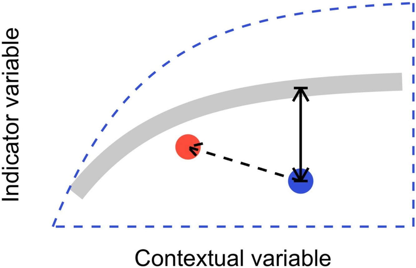
In this letter, we propose that level-2 ecological integrity could be conceptualized as the departure from a reference relationship between an indicator variable of interest and a contextual variable that describes the situation-dependent state of an ecosystem, including its level-1 ecological integrity. Departure from the reference should identify ecosystems that are more or less efficient structures than the average standard. Once such relationships have been described (see next section), level-2 ecological integrity can be measured in terms of deviations relative to this reference. Ecosystems further from the reference relationship are those that require our immediate attention in an analogy to a triage system. Additionally, it provides an objective measure to determine if the state of an ecosystem is degrading or improving over time (Fig. 1).
 from the reference relationship. Red point and corresponding dashed arrow is a possible trajectory the ecosystem could take, where despite a change of context, its level-2 integrity (deviation from the reference relationship) would improve.")
Conceptual model of level-2 ecological integrity assessment from the standardization of an indicator variable with a contextual variable. Dashed blue line is the envelope enclosing all possible ecosystem states. Thick gray line is the reference relationship. Blue point is a particular ecosystem, with a particular deviation (its level-2 integrity deficit) from the reference relationship. Red point and corresponding dashed arrow is a possible trajectory the ecosystem could take, where despite a change of context, its level-2 integrity (deviation from the reference relationship) would improve.
Plant biomass accumulation is a variable of primary interest that controls the fluxes of fundamental elements on Earth. For plant biomass to accumulate, a community needs sufficient light, water and nutrients, as well as an appropriate species pool to take advantage of the local conditions. Biomass changes are thus synthetic measures for all these biotic and abiotic constraints. Since aboveground plant biomass is structurally limited by plant height, and plant height is conditioned by disturbance regime, development stage and resource limitation (light, water, nutrients, etc.), the environmental context could be accounted for once biomass accumulation is standardized for stand height. In this framework, plant stand height becomes our contextual variable (how big are the plants here?) and aboveground biomass our indicator variable of interest (how much carbon the plant stand stores?). The standardization of mass by height for any plant community would provide a measure of biomass packing; that is, the amount of aboveground plant material that can be packed per unit volume.
We investigated the generality of the relationship between the height of vegetation stands and their aboveground dry biomass, to assess its potential as a level-2 ecological indicator. From a dataset of 971 plant stands gathered from 12 studies around the globe (see Proulx et al., 2015 for dataset details), we showed that both community biomass and height are dependent on their specific environmental context (Fig. 2). Nonetheless, when looking at the global relationship between these two commonly measured variables, one finds a consistent relationship (Fig. 3), suggesting that the amount of aboveground plant biomass is constrained by the stand height. An earlier assessment of biomass packing showed that ratios above 5 kg m−3 are probably not sustainable by natural communities, implying the existence of a limiting envelope to the relationship (Proulx et al., 2015, dashed blue line in Fig. 3).
 biomass (kg m−2) and (b) community height (m) in 971 plant communities gathered from 12 studies around the globe. Boxes contain 50% of the data, with center line at median. Whiskers extend up to 1.5 interquartile range.")

Relationship between community stand height and aboveground biomass in 971 plant communities gathered from 12 studies around the globe in 5 ecosystem types. Biomass is measured in dry kg m−2, community height is in m. Dashed blue line is the maximum achievable aboveground biomass for a given stand height in natural communities.
A preliminary assessment of the biomass packing suggests that the height-biomass relationship of vegetation stands is also robust across both air temperature and soil fertility gradients (Proulx, submitted). This implies that, irrespective of the environmental or naturalness context, processes that enable coexistence may constrain the amount of aboveground plant biomass stored per unit volume (Proulx et al., 2015). Biomass packing (the standardization of aboveground biomass by stand height) could provide an easily measurable index of the efficiency of a plant community at storing carbon in aboveground tissues. A similarly general, strong and linear relationship between aboveground biomass and plant height was revealed on an independent dataset of 75 vegetation stands from different environmental contexts (Franco and Kelly, 1998).
Although promising, the biomass packing relationship also presents some limitations, which must be accounted for appropriately. For instance, competition for resources can affect aboveground biomass and densities only in crowded plant communities. Biomass and stand height measurements thus need to be conducted at peak biomass, and cannot be used for year-round assessments, especially in climates with strong seasonality. Moreover, trees in younger stands tend to invest in height and only later, once the stand has matured, in trunk diameter (Henry and Aarssen, 1999). The latter phenomenon probably explains the clump of less efficient forest communities which are entering the reference relationship from below in our example (Fig. 3). Biomass packing is therefore sensitive to the definition of plant height, and care must be taken to measure canopy height in relatively homogenous stands.
At the landscape scaleAt a larger scale, the “state” of landscapes can also be described in terms of reference relationships. One simple indicator variable at this scale is habitat connectivity (e.g. patch size, edge density). Changes in habitat connectivity may occur naturally, through disturbances, biome transitions, landform changes, or because of human-driven modifications to the landscape. Ecology has a long tradition of studying the impacts of habitat connectivity on populations and communities, going back to debates on the optimal spatial organization of natural reserves (Diamond, 1976, the SLOSS debate; 1975; Simberloff and Abele, 1976, etc.), to processes underlying the maintenance of species in patchy habitats (Levins, 1969; Pulliam, 1988; Wilson, 1992).
Habitat connectivity is strongly related to the amount of (semi-)natural habitat in the landscape, as any removal (or addition) of habitat changes the configuration of the patches. Habitat amount in this sense is usually defined as the area of land cover that can fulfil some species’ needs. In many cases, the amount of habitat is interpreted as (and often confounded with) the amount of natural cover remaining in the landscape, although fundamentally, one species’ inhospitable matrix can be home to another one. Some authors have nevertheless questioned whether habitat connectivity has effects on biodiversity that are independent of habitat amount (Fahrig, 2013; Martin, 2018). To account for differences between landscapes in different environmental contexts, mean patch size (the variable of interest) must be standardized by the amount of habitat (the contextual variable).
Very few authors have tested how strongly the mean patch size of habitats is tied to habitat amount in existing landscapes (Didham et al., 2012; but see Proulx and Fahrig, 2010). To assess the usability of this indicator as a level-2 ecological integrity measure, we built a dataset to assess the strength and generality of the mean patch size-habitat amount relationship. We randomly selected 10,000 square landscapes of 25 km2 anywhere in the continental USA from the 2001 National Land Cover Database (NLDC, Homer et al., 2015). Random landscape coordinates were selected from a uniform distribution bounded by the latitude and longitude range of the continental USA. Landscapes consisting entirely of water were discarded during the sampling process. In each landscape, we calculated the forested area (a one-sided view of habitat amount) and the average size of forest patches (a measure of habitat connectivity). Similar definitions of habitat amount are widespread in the landscape ecology literature. We then re-inspected every landscape in the 2011 NLCD to explore the dynamics of this relationship ten years later.
By studying thousands of landscapes across the continental US, irrespective of their specific environmental context, a clear pattern emerges (Fig. 4). Habitat amount during this 10-year period is decreasing in most landscapes, as indicated by the direction of arrows. Yet, a surprisingly constrained relationship remains between habitat amount and mean patch size. There seems to exist a narrow amount of connectivity (i.e. mean patch size) that landscapes reach for a given amount of habitat, despite the variety of forces that act upon landscape development (e.g. Antrop, 1998). The constraints are particularly strong when considering the range of configuration patterns that man or nature could possibly achieve for a given amount of habitat (Fig. 4, dashed blue line forming the bottom of the envelope).
 and mean patch size (ha) in 10,000 randomly selected 25 km2 landscapes across the continental USA. Arrows point from the 2001 configuration to the 2011 configuration of each landscape. Dashed blue line is the envelope defining all the possible configurations a landscape could take, limited at the top by a single patch using all the forested area, and at the bottom a checkerboard-like pattern forming as many habitat patches as possible for a given forested area.")
Relationship between habitat amount (forested area; ha) and mean patch size (ha) in 10,000 randomly selected 25 km2 landscapes across the continental USA. Arrows point from the 2001 configuration to the 2011 configuration of each landscape. Dashed blue line is the envelope defining all the possible configurations a landscape could take, limited at the top by a single patch using all the forested area, and at the bottom a checkerboard-like pattern forming as many habitat patches as possible for a given forested area.
With our general reference relationship in hand, we can now look at it as a level-2 integrity indicator (mean patch size standardized by habitat amount). Although it is clear that protecting more habitat is a reasonable conservation target (level-1 ecological integrity), different landscapes in contrasted environmental or naturalness contexts can be compared when looking at the deviation of mean patch size from the reference relationship. Considering that the relationship generalizes across different contexts, one can independently assess if patches are too small for the amount of habitat that remains in the landscape. Using different measures of habitat amount and connectivity, Proulx and Fahrig (2010) found a strong and general relationship between the two measures for landscapes all across Canada. Deviations from this relationship indicated that the process of agricultural development leads to a reduction in pattern variation (Proulx and Fahrig, 2010).
DiscussionLevel-2 metrics of ecological integrity could be applied to prioritize conservation and restoration efforts in novel, more nuanced ways. For example, the city council of a suburban town votes on a budget to improve the ecological integrity of one of its parks, and has to decide which one to restore. One park is in a downtown area. It is mostly concrete structures with few small patches of trees. The other park is in a forested area near the edge of the town and has more, and larger, patches of trees. For analysis purposes, we will consider these parks as small landscapes of equal size. Based on connectivity measurements (level-1 assessment), the downtown park would be the obvious restoration target, being the less natural one with smaller, less connected tree patches. On the other hand, level-2 metrics (i.e. standardized mean patch area per natural habitat amount) might point out that the forested park is the most in need of restoration, because compared to other parks with similar amounts of tree cover, the patches in this one are smaller. In this context, the level-1 and level-2 metrics would provide two different pieces of information. Level-1 informs us about how natural an ecosystem is, whereas level-2 helps us assess how modified an ecosystem is compared to others in similar contexts. Without level-2 assessment, the forested park might not see any restoration work before its tree cover is as sparse as the downtown one.
One drawback of using contemporary data points to construct reference relationships is that the current situation is considered as normal. It also means that the relationship between level-1 and level-2 indicators of integrity is dynamic, and may continue to shift through time. If humanity keeps altering ecosystems more and more, the target for a typically connected landscape will only get lower and lower. This moving target should be taken as a reminder that we ultimately control the fate of ecosystems on Earth. It is, again, all about priority management.
Through refining the set of reference relationships to the point where they are useful to compare ecosystems and set management priorities, conservationists will also be facing novel moral dilemmas. By using an objective level-2 measure of ecosystem state, we put aside considerations about the presence of particular habitat structures, species, or communities of special interest. For example, if a popular recreational hunting species is declining and our integrity assessment indicates there is nothing particular to worry about, what should we do? Should we actively manage the ecosystem to preserve the species? Recognizing such circumstances will force us to be upfront about our motivations for protecting species or ecosystems of interest. We may need to acknowledge that sometimes we protect nature simply because we appreciate and value it (Vellend, 2017).
ConclusionOnce Noah’s Ark is full and we have saved some of nature’s wonder, future management priorities will need to focus on ecosystems under moderate stress and disturbance. The more transformed and managed ecosystems are, the less useful level-1 assessment measures will become. The clock is ticking for scientists to develop level-2 measures of ecosystem integrity that are applicable in different ecosystems and environmental contexts. We believe that conservation research should focus on describing and testing widely applicable standardizing relationships in order to objectively set targets for level-2 ecosystem integrity. Rehashing the current pristine-or-anthropized indicators over and over could, before long, cause ecologists to lose the few sympathetic ears we have today.
Declaration of interestsThe authors declare that they have no known competing financial interests or personal relationships that could have appeared to influence the work reported in this paper.
This research was supported by grants from the Natural Sciences and Engineering Research Council of Canada and the Canada Research Chair Program to R. Proulx. R. Proulx would also like to thank Lael Parrott for her input through the conceptualization of this article. We are grateful to an anonymous reviewer for their helpful comments.

