


Epidemiology is one of many fields that use ecological niche modeling to assess potential distributions or potential range expansions of species. When such models are transferred in space and time, it is important to understand sources and location of uncertainty in their predictions. Here, we used the tick species Rhipicephalus sanguineus sensu lato (distributed in different areas around the world) as an example; for the first time, we characterized its global geographic distribution using ecological niche modeling, and explore the uncertainty involved in transferring models in space and time. We assessed uncertainties based on risks of strict extrapolation and amounts and patterns of variation in our predictions. We integrated occurrence records and climate data to calibrate models for 5 world regions, and to project them to 11 general circulation models (GCMs) and two representative concentration pathway emissions scenarios (RCPs) for 2050. Models created in different calibration areas showed high agreement of suitable areas among model predictions from the eastern United States, southern Mexico, South America, Europe, North Africa, sub-Saharan countries, Asia, and Australia. The global potential distributions of R. sanguineus sensulato were very similar between the two RCPs, but GCMs, model replicates, and model parametrizations contributed importantly to the overall variation detected. Patterns of uncertainty (strict extrapolation areas and variation) in our model predictions depended on the calibration area, and underlined the important implications of not considering variability and extrapolation risk in interpretations of ecological niche model projections.
Thanks to Joseph Grinnell, who explored relationships between geographic distributions and ecological niches (Grinnell, 1917), the foundations for the modern idea of ecological niche modeling (ENM) were laid. ENM uses environmental characteristics of known occurrence sites for species to understand the environmental conditions under which the species can maintain populations at a site without immigrational subsidy (Peterson et al., 2011). Considering disease risk mapping, ecological niche models are important tools in characterizing potential geographic distributions of hosts (Samy et al., 2016a), vectors (Alkishe et al., 2017; Kamal et al., 2018; Raghavan et al., 2019a), human cases (Levine et al., 2007), or pathogens (Peterson, 2006), under current and future conditions.
In disease biogeography, various frameworks have been explored to translate distributional understanding into maps of transmission risk (Peterson, 2014). Nonetheless, in disease mapping, ENM comes with caveats in both biodiversity conservation and public health, and any wrong information can have negative implications for human and animal health, and animal conservation programs (Escobar and Craft, 2016; Peterson and Vieglais, 2001). Since ENM outputs include uncertainty from several sources (Petchey et al., 2015; Peterson et al., 2018), rigorous model calibration processes and measurement of certainty or uncertainty are crucial when performing these exercises (Cobos et al., 2019a).
Ticks are disease vectors that transmit pathogens to many animal species, including livestock and humans (Dantas-Torres et al., 2017). Rhipicephalus sanguineus sensu lato (Acari: Ixodidae), or the brown dog tick, has been reported in different regions of the world, so even the native area for this species is not clear (TISI, 2014). It is the vector of various etiological agents for dogs and humans, such as Rickettsia conorii, R. rickettsii, Coxiella burnetii, and Ehrlichia canis (Dantas-Torres, 2010b). Rhipicephalus sanguineus sensu lato differs from most ixodid ticks in terms of its behavior: whereas most are exophilic (i.e., they tend to rest outdoors), R. sanguineus sensu lato has the ability to complete its life cycle as exophilic or endophilic (i.e., it can be found indoors). This characteristic can help this species to establish and maintain populations in colder areas, and also increases its biting rate (Dantas-Torres, 2008). Although the endophilic behavior may allow some buffering against seasonal climate effects, climate clearly does impose limits at some point on the distributional potential of this species.
Rhipicephalus sanguineus sensu lato can spread Rocky Mountain spotted fever (RMSF) by transmitting Rickettsia rickettisii to humans (Drexler et al., 2014). During 2003–2012, at least 250 RMSF cases were reported, and 19 deaths were registered in Arizona’s Native American communities (Herrador et al., 2017). Rhipicephalus sanguineus sensu lato can also spread Rickettsia conorii which causes Mediterranean spotted fever (MSF), endemic in many countries in southern Europe and North Africa (Gomez-Barroso et al., 2019; Parola et al., 2009). Recently, MSF cases have been reported in new regions, such as central Europe, central and southern Africa, and countries around the Black Sea (Bulgaria, Ukraine, and Turkey) (Rovery et al., 2008). In Spain, for instance, 4735 MSF cases were diagnosed during 1997–2014, with most cases in the summer season (Herrador et al., 2017). Males of Rhipicephalus. sanguineus sensu lato have the ability to move from dogs to the environment, and then to humans, which could promote transmission of pathogens between species (Little et al., 2007). Rhipicephalus. sanguineus sensu lato is known to maintain populations under a broad range of conditions: e.g., temperatures of 20−35 °C and humidity of 35-95% (Dantas-Torres et al., 2011; Parola et al., 2008; Yoder et al., 2006), so climatic variables may be important predictors of Rhipicephalus. sanguineus sensu lato’ distribution, and changes in these variables may affect populations of this species significantly.
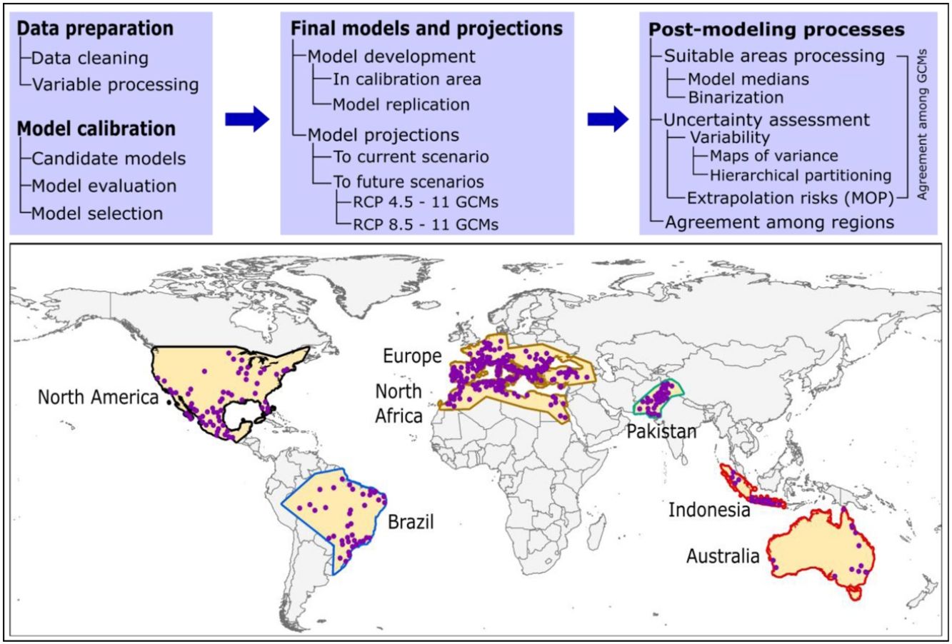
Here, we used ecological niche modeling to characterize R. sanguineus sensu lato environmental requirements as regards aspects of temperature and precipitation and potential geographic distribution under present and future conditions in different regions. Most importantly, we also assessed uncertainty in terms of model variability coming from distinct sources and of risk of strict extrapolation in model transfers associated with model outputs. We present this analysis as both a first global assessment of the species’ distributional potential, and an illustration of how best to assess and understand uncertainty ecological niche models of public-health-important species (see analysis workflow in Fig. 1).
MethodsInput data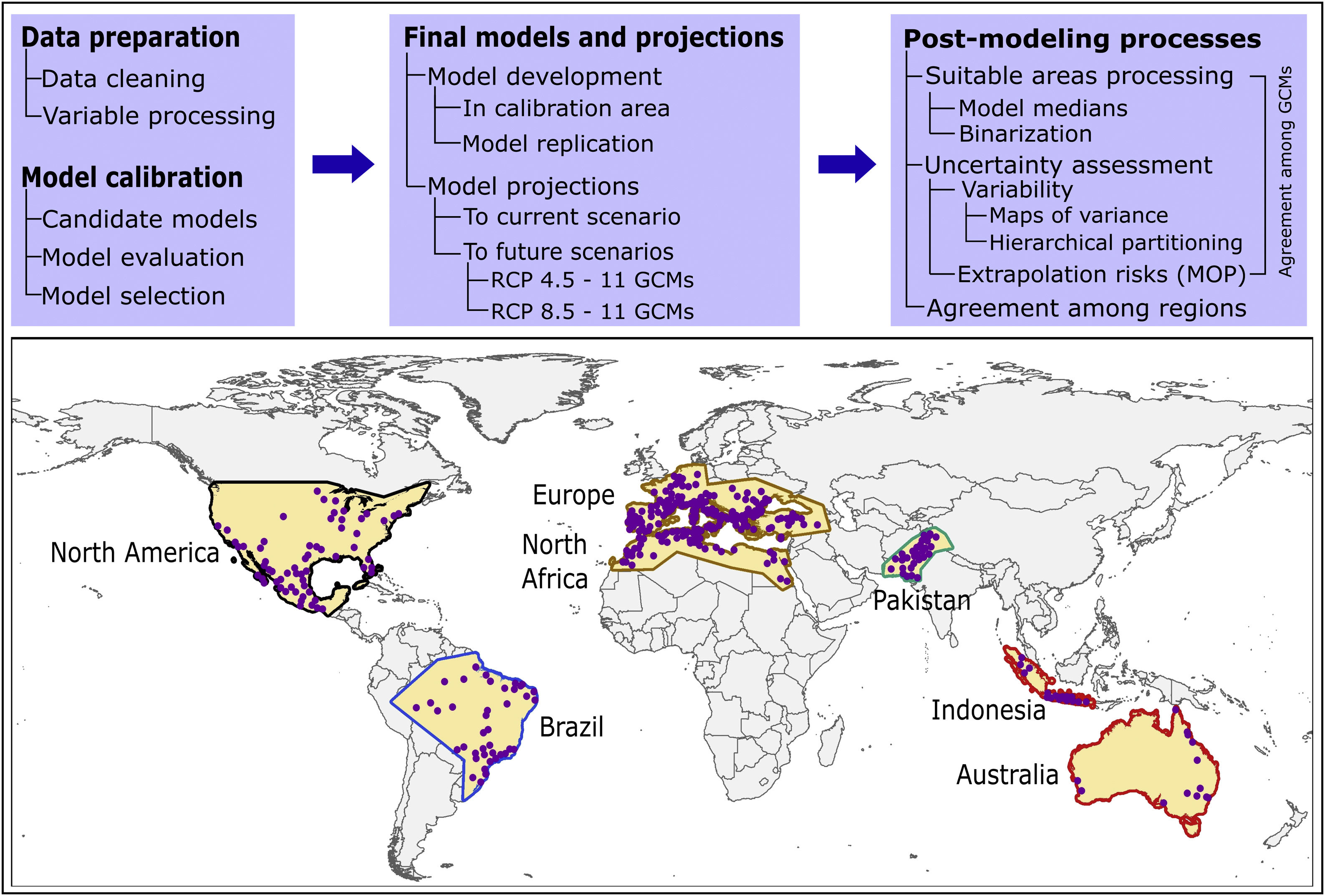
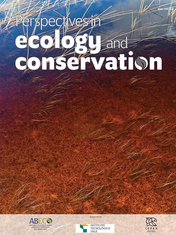
Occurrence data for R. sanguineus sensu lato were compiled from the Global Biodiversity Information Facility (GBIF; www.gbif.org; 8189 occurrence points), SpeciesLink (http://www.splink.org; 430 occurrence points), and the scientific literature (746 points; Appendix S1 File) (Estrada-Peña et al., 2016). Occurrence points were clustered in 5 regions on different continents of the world, and were highly clumped as a consequence of biases in sampling and reporting (Fig. 1). We undertook several data cleaning steps to reduce potential bias in the occurrence dataset (9365 records in total) (Cobos et al., 2018; Syfert et al., 2013). Data cleaning steps included the following: (1) review and assessment of potential taxonomic mistakes in the database, removing records likely not corresponding to the taxon in question; (2) removal of occurrences lacking geographic references, records with (0, 0) for geographic coordinates, records in the ocean and seas, and duplicate records; and (3) relocation (to the closest pixel) of records that were on the sea but close to the coast (i.e., errors related to pixel resolution).
Semivariogram analysis was used in ArcGIS 10.5.1 to determine the reasonable distance to reduce clustered occurrence points. The remaining points were thinned (i.e., spatially rarefied) with a 50 km distance filter in ArcGIS 10.5.1, using the SDMtoolbox [version 1.1c; (Brown, 2014)]. The specific distance used to thin occurrences was selected based on the spatial resolution of environmental variables (see below), the environmental heterogeneity present in areas where the species is known to be distributed, and the precision and accuracy of the available occurrence data for the species. Since the density of occurrences was overly high in some sub regions, which could end in overfitted models that underestimate species potential distributions—we randomly reduced the number of records in areas where densities were too high following (Raghavan et al., 2019b). After all these steps, we obtained a final set of 368 occurrences of R. sanguineus sensu lato (see details in Appendix S2 File); these data were subset randomly into two groups, 50% for training and 50% for evaluating model predictions.
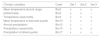
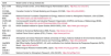
We used 15 of the 19 so-called “bioclimatic” variables obtained from the WorldClim database (version 1.4) at 10′ resolution (∼20 km; available at www.worldclim.org); such variables derive from interpolation of average monthly temperature and rainfall data (Hijmans et al., 2005). Four variables combining information of temperature and precipitation were removed (variables 8, 9, 18, and 19) owing to known spatial artefacts (Broennimann et al., 2012; Samy et al., 2016b; Samy and Peterson, 2016). We used iterative jackknife procedures in Maxent 3.4.1 (Phillips et al., 2017, 2006) for identifying three candidate sets of predictors, as having various candidate sets of variables has been suggested to improve the process of model calibration (Cobos et al., 2019b). Variables were selected considering their contribution to models and their collinearity (these procedures were implemented across the entire area of model calibration, see below). When two or more variables were correlated (r ≥ 0.8), we selected the one with the highest contribution and excluded the others. Final sets of variables included 7 variables in set 1, 6 in set 2, and 5 in set 3 (Table 1).
Environmental variables used in ecological niche model calibration. Source: WorldClim (Hijmans et al., 2005).
| Climatic variables | Code | Set 1 | Set 2 | Set 3 |
|---|---|---|---|---|
| Mean temperature diurnal range | Bio2 | x | x | x |
| Isothermality | Bio3 | x | x | – |
| Temperature seasonality | Bio4 | x | x | x |
| Mean temperature of warmest quarter | Bio10 | x | x | x |
| Annual precipitation | Bio12 | x | – | – |
| Precipitation seasonality | Bio15 | x | x | x |
| Precipitation of driest quarter | Bio17 | x | x | x |
To represent future climatic conditions, we used the bioclimatic variables for 2050 representing outputs of 11 general circulation models (GCM) in two representative concentration pathway emission scenarios (RCP 4.5 and RCP 8.5; Table 2). RCP 4.5 represents a scenario of medium-low greenhouse gas (GHG) concentrations, whereas the RCP 8.5 scenario represents high levels of GHGs in the future (Stocker et al., 2013). The GCMs represent independent simulations of global processes that translate into climate. These models can be applied to greenhouse gas concentrations expected under different RCPs to reduce detailed scenarios of future conditions. Future scenarios were obtained from Climate Change, Agriculture and Food Security (CCAFS; available at http://www.ccafs-climate.org/data_spatial _downscaling).
General circulation models explored in this analysis, each with data for two distinct emissions scenarios, RCP 4.5 and RCP 8.5.
| GCM | Model Center or Group (Institute ID) |
|---|---|
| BCC-CSM 1−1 | Beijing Climate Center, China Meteorological Administration (BCC; http://bcc.ncc-cma.net/) |
| CCCMA-CANESM2 | Canadian Center for Climate Modeling and Analysis (CCCMA; https://bit.ly/2AxSQN3) |
| CESM1-BGC | National Science Foundation Department of Energy, National Center for Atmospheric Research, USA (CESM1; http://www.cesm.ucar.edu/models/cesm1.0/) |
| CSIRO-MK 3−6-0 | Commonwealth Scientific and Industrial Research Organization (CSIRO) and Bureau of Meteorology (BOM), Australia; https://www.csiro.au/en/Showcase/state-of-the-climate. |
| GISS – E2 - R | NASA Goddard Institute for Space Studies (NASA GISS), USA; https://www.giss.nasa.gov/ |
| INM-CM 4 | Institute for Numerical Mathematics (INM), Russia; http://www.inm.ras.ru/ |
| IPSL-CM5A-MR | Institute Pierre-Simon Laplace (IPSL), France; https://www.ipsl.fr/en/ |
| MIROC 5 | Atmosphere and Ocean Research Institute (University of Tokyo), National Institute for Environmental Studies, and Japan Agency for Marine-Earth Science and Technology (MIROC); https://bit.ly/2ZXQcK9 |
| HadGEM 2-ES | Met Office Hadley Centre (MOHC), UK, with contribution from Instituto Nacional de Pesquisas Espaciais (INPE), Brazil; https://bit.ly/2JeSiPd |
| MRI – CGCM 3 | Meteorological Research Institute (MRI), Japan; http://www.mri-jma.go.jp/index_en.html |
| CCSM 4 | National Center for Atmospheric Research, USA (NCAR); https://bit.ly/2NpvYaQ |
In view of the broad geographic distribution of the species in question, we delimited the area for calibrating models as the portion of the countries that has been potentially accessed by the species and has been sampled by researchers (Barve et al., 2011; Peterson, 2014). This process resulted in five disjunct regions (North America; Brazil; Europe and North Africa; Pakistan; and Indonesia and Australia; Fig. 1). We used randomization tests of niche similarity [i.e., background similarity tests; (Warren et al., 2010)] among occurrences in the five regions to determine whether models should best be developed using the whole dataset or based on each region separately. These analyses assess whether observed levels of similarity of occupied sites between regions are sufficiently low when compared to a null distribution of region-to-region similarity values that a null hypothesis of niche similarity can be rejected.
The background similarity tests were performed with 1000 replications, using routines implemented in the ENMTools R packages (Broennimann et al., 2012; Warren et al., 2010). The background similarity test is performed based on similarity between the areas identified as suitable compared with random areas from across the calibration area (i.e., it is performed in geographic space). This test generates two results as it is a two-way analysis. The similarity (Schoener’s D index) between actual models is compared with similar indices calculated between models generated from random samples from across the calibration area, and then repeated in the opposite direction (Warren et al., 2010). The similarity test (Broennimann et al., 2012) is performed using the environmental values in the species occurrences and in the calibration area; when environments of calibration areas are not similar at all, the test has no statistical power; this analysis is performed in the environmental space.
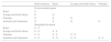
Given the outcome of the similarity tests (Table 3), we decided to calibrate distinct models in six calibration areas: each of the five calibration areas and the union of all five. We tested a total of 1479 candidate models created using Maxent under distinct settings, resulted from combinations of three sets of environmental variables, 29 feature classes (all combinations of linear = l, quadratic = q, product = p, threshold = t, and hinge = h), and 17 regularization multiplier values (0.1–1 at intervals of 0.1, 2–6 at intervals of 1, and 8 and 10). These models were evaluated based on statistical significance (partial ROC; (Peterson et al., 2008)), predictive ability (omission rates, E = 5%; (Anderson et al., 2003)), and complexity (Akaike information criterion corrected for small sample sizes, AICc (Warren et al., 2010)). Best parameterizations were chosen among the significant models that had omission rates below 5% and delta AICc values lower than two. All calibration exercises (candidate model creation, evaluation, and selection) were conducted in the kuenm R package (Cobos et al., 2019a) available at https://github.com/marlonecobos/kuenm).
Results of niche similarity tests in geographic space (Geo) (Warren et al., 2010) and environmental space (Env) (Broennimann et al., 2012). X indicates significant results (non-similar niches); O indicates non-significant results (no evidence to reject similarity). Entries for results in geographic space are double as this analysis is bidirectionally (see Methods).
| North America | Brazil | Europe and North Africa | Pakistan | ||||
|---|---|---|---|---|---|---|---|
| Environmental space | |||||||
| Brazil | X | ||||||
| Europe and North Africa | O | O | |||||
| Pakistan | O | O | O | ||||
| Australia and Indonesia | O | X | O | O | |||
| Geographical space | |||||||
| Brazil | X - X | ||||||
| Europe and North Africa | X - X | X - X | |||||
| Pakistan | X - X | X - X | O - X | ||||
| Australia and Indonesia | X - O | O - O | X - X | X - X | |||
For each calibration area in which good models were obtained (i.e., significant, low omission, and simple models), we created final models using the complete set of occurrences and the parameterizations selected during model calibration. We performed 10 replicates by bootstrap and transferred the models globally in current and future climate scenarios, calculated medians of the 10 replicates were used as final predictions for each calibration area. We binarized models based on a fixed allowable omission error rate of 5% among calibration data (Anderson et al., 2003), assuming that up to 5% of the occurrence data may have included errors that misrepresented environments used by the species, which is appropriate when input data are heterogeneous and uncontrolled in origin (Peterson et al., 2008). For current-time predictions, we present suitable areas produced with the union of data from all calibration areas (5 regions), and also a summary of agreement of suitable areas produced with data from each calibration area separately. For each future scenario (RCP 4.5, and 8.5), we calculated differences in suitability between current and future scenarios (median across parameter settings), and represented agreement of predictions of changes of suitable areas (stable, gain, loss) among the 11 GCMs used. Gain refers to presently unsuitable areas anticipated to become suitable in the future. Loss, on the contrary, refers to currently suitable areas not suitable under future conditions. Final models, their transfers, and other post-modeling analyses were developed using the kuenm R package.
Model uncertaintyWe evaluated model uncertainty by detecting areas of strict extrapolation (Owens et al., 2013), and estimating the amount and patterns of variation coming from distinct sources in model projections. Areas of strict extrapolation in model projections are places where environmental conditions are non-analogous to those in areas across which the models were calibrated. To identify such extrapolative areas, we used the mobility-oriented parity metric [MOP nearest 5% of reference cloud; (Owens et al., 2013)]. This method evaluates levels of similarity between calibration and projection areas, and identifies areas of strict extrapolation based on calculated similarities. In one explanation, we excluded suitable areas where strict extrapolation existed in our maps to represent only potential distributional areas with higher levels of certainty. MOP analyses were performed for the area resulting from the union of all calibration areas and for each of the four calibration areas (excluding one for which no useful models were available, compared with conditions worldwide under current and future climate scenarios using the kuenm R package.
Variation coming from distinct sources was evaluated in two distinct ways, following (Peterson et al., 2018), and (Cobos et al., 2019b). First, we performed a hierarchical partitioning analysis of sources of variance in model geographic projections (Diniz‐Filho et al., 2009; Terribile et al., 2012) considering replicates, parameter settings, GCMs, and RCPs as factors, although we note that not all calibration areas have all sources of variation because for some calibration areas only one set of parameters was selected (Peterson et al., 2018). Second, we created maps illustrating the amount of variation coming from different sources to understand geographic patterns associated with each of these factors (Peterson et al., 2018). These two processes were also performed using kuenm.
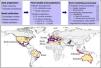
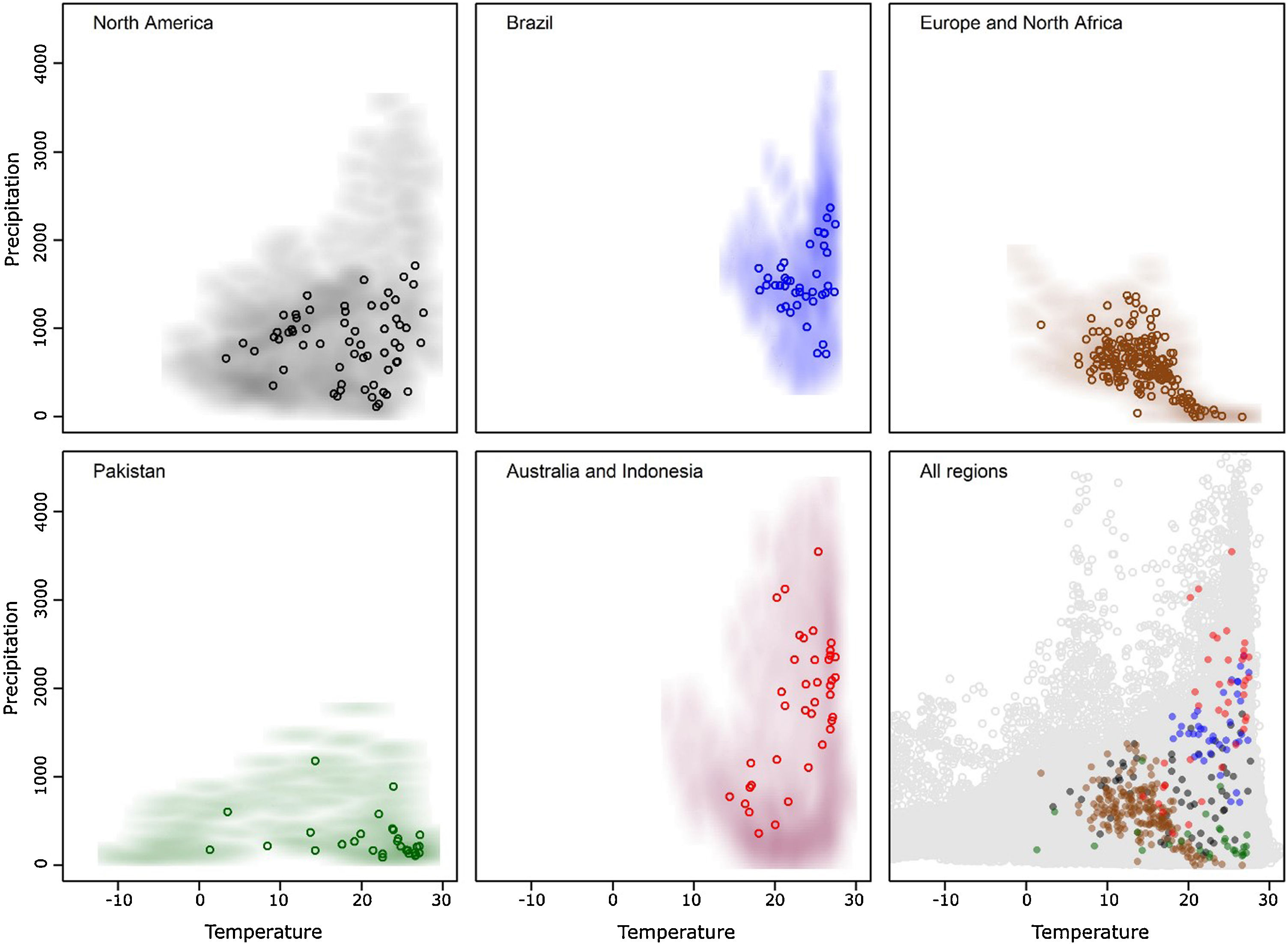
ResultsAfter data cleaning, we had 368 occurrence points from our initial total of 9365 for R. sanguineus sensu lato (Fig. 1). The arrangement of occurrences in environmental space in the five regions showed the species to be distributed differently in temperate and tropical environmental conditions in the four distinct regions (Fig. 2). The background similarity tests showed that most regional comparisons were significant in geographic space, indicating niche differences, but only two comparisons were significant in environmental space (Table 3), such that evidence for niche differentiation was mixed.
In terms of environmental variable sets, models for North America, Europe and North Africa, and Indonesia and Australia, performed better with the five environmental variables in set 3; in Brazil, models performed well with all 3 environmental variable sets, and the global analysis was best based on the 7-variable dataset (Appendix S2 File). Although we had a good sample (31 points) from Pakistan, the model prediction did not perform better than random expectations, and omission rates were too high (all model omission rates > 0.1) in this calibration area so we excluded Pakistan from our analyses. Model predictions in other calibration areas were significantly better than random expectations (P < 0.05; Appendix S3 File).
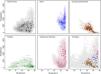
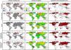
Current predictionsThe global model (the one calibrated in all calibration areas together) predicted broad suitable areas for the species around the world (Fig. 3A), including broader suitable areas in North America, South America, and Europe and North Africa than models based on each calibration area separately (see Fig. 3E). Models based on each calibration area separately showed the potential geographic distribution of R. sanguineus sensu lato under current-day conditions with high agreement across the eastern United States, southern Mexico, northern South America, Brazil, Europe, North Africa, sub-Saharan countries, Asia, and Australia (Fig. 3E).
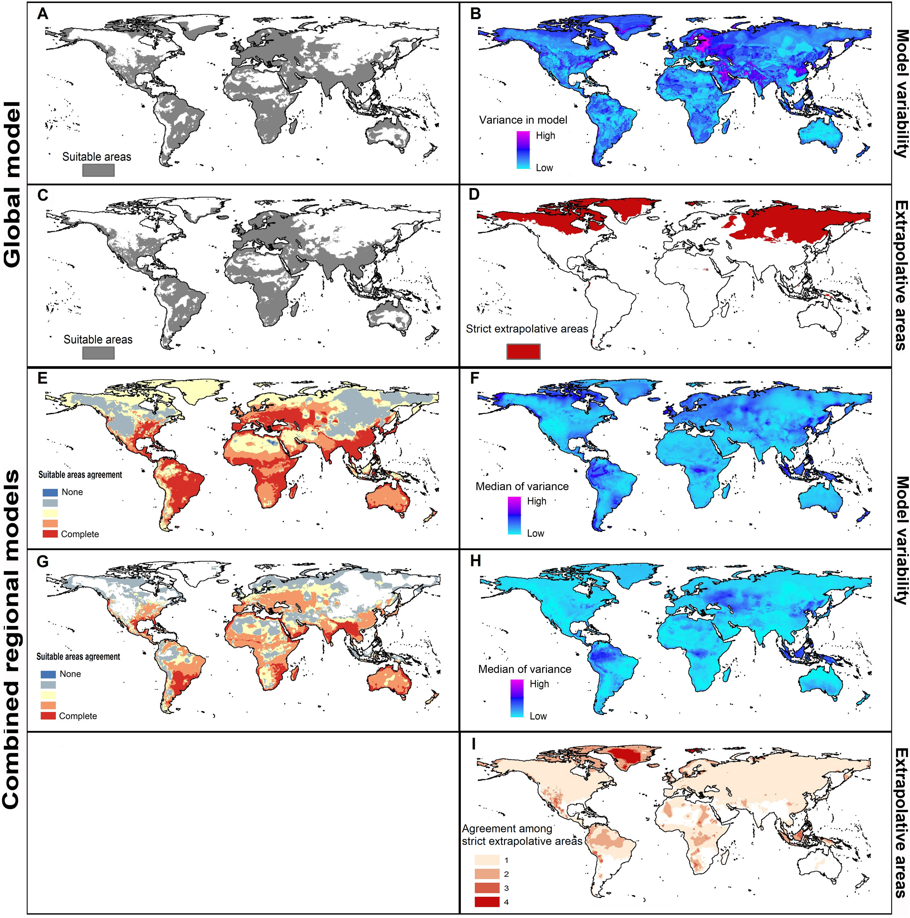
Potential distribution of Rhipicephalus sanguineus sensu lato based on present-day conditions. Left panels show model outcomes; right panels show model variability. A. Current suitable including areas of strict extrapolation. B. Variance in model in current projection coming from replicates. C. Current suitable without strict extrapolation areas. D. Areas of strict extrapolation. E. Agreement among suitable areas created with the 4 regions of calibration including areas of strict extrapolation. F. Median of variance from replicates in current projections of models created with 4 calibration regions. G. Agreement of current suitable areas predictions excluding areas of strict extrapolation. H. Median of variance from parameters in current projections of models created with 4 calibration regions. I. Agreement among areas of strict extrapolation from the 4 calibrations regions.
MOP results showed areas of strict extrapolation mainly in the Northern Hemisphere (Fig. 3D and 3I) and some other areas around the world (Fig. 3I) when looking at results for all calibration areas combined and at agreement among them. Removing areas of strict extrapolation, northernmost suitable areas were excluded for models created with combined calibration areas (Fig. 3C) and the degree of agreement among models for the four calibration areas was reduced (Fig. 3G). High levels of agreement among reduced suitable areas from the four models were found in the southeastern United states, southern Brazil, North Africa, eastern South Africa, along the Red Sea, southern Asia, and in Australia; additional areas in Central Europe, Brazil, sub-Saharan Africa, Australia, and some parts of the eastern United States and North Africa showed medium-to-high levels of agreement (see Fig. 3).
In current predictions of global models, all variation came from replicates (Fig. 3B) since only one parameter setting was selected as the best. Maximum levels of variation in global models were in northeastern Europe, the Middle East, and parts of Greenland, Pakistan, India, and China. When calibration areas were analyzed separately, levels of variation were similar between replicates and parameters in current predictions (Fig. 3F and 3 H). Variation from replicates (Fig. 3F) showed variation concentrated in the Northern Hemisphere, western South America, and parts of sub-Saharan Africa, Indonesia, and Malaysia. Variation from parameter settings was concentrated in a few areas of Eastern Europe, western South America, Indonesia, and Malaysia (Fig. 3H).
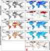
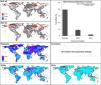
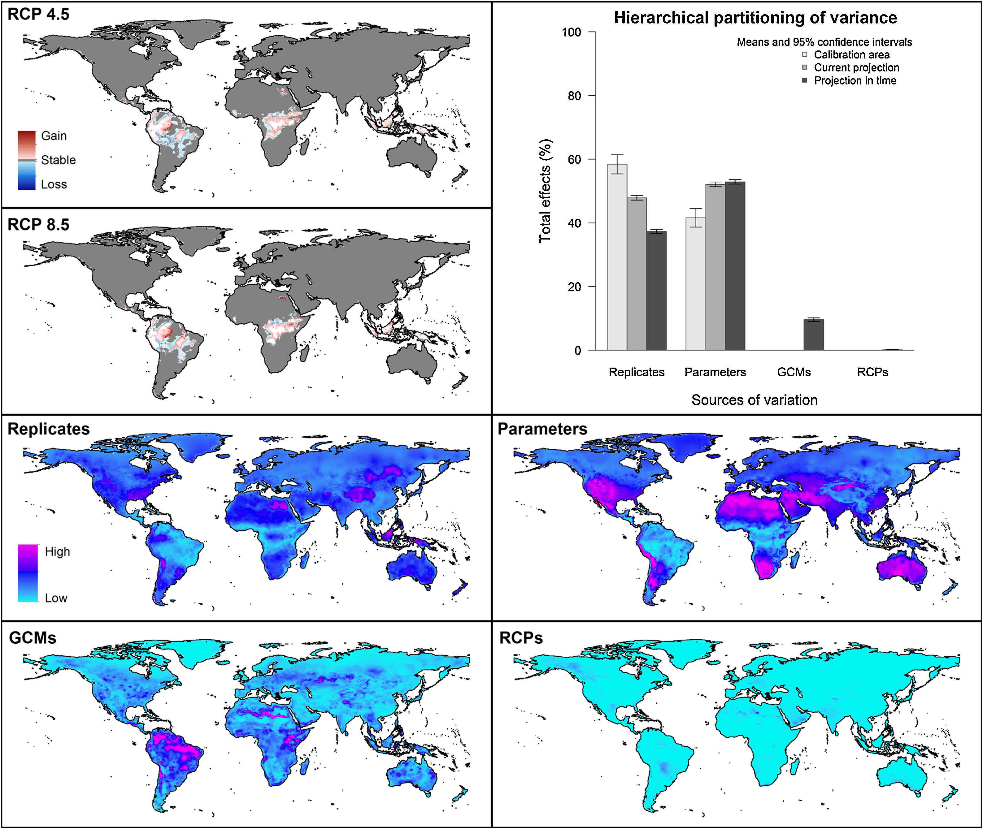
Future predictionsFor global-calibration models transferred to conditions in 2050, under RCP 4.5 suitable areas were predicted to be stable across large areas of Europe, southern Asia (China, India, Indonesia), northern Australia, and parts of sub-Saharan Africa and northern North America (Figs. 4 and 5 and Appendix S4 File.). Some newly suitable areas were observed in the Northern Hemisphere, such as in Russia and Canada, as well as in North Africa and parts of Australia. Losses of suitable areas were somewhat higher in RCP 4.5 than RCP 8.5, especially in South America. Future increases in suitability were detected mainly in the Northern Hemisphere; decreases were distributed worldwide, somewhat concentrated in the eastern United States and southern Europe (Fig. 4 and Appendix S4 File).
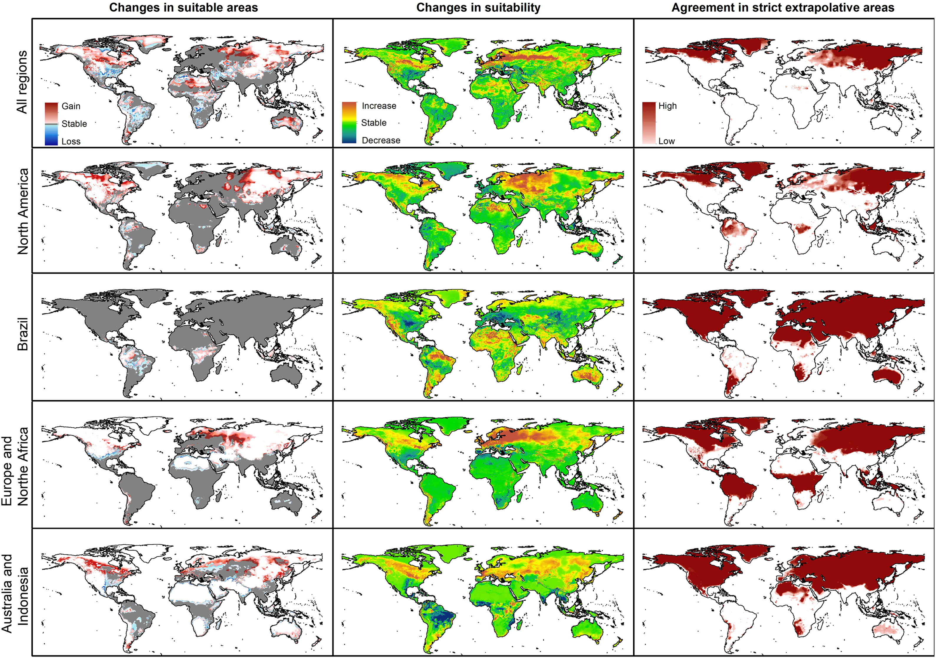
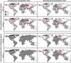
For single-region models, under future conditions, suitable areas were projected to remain stable largely worldwide for models calibrated in North America, Brazil, and Europe; for models calibrated in Australia, suitable areas were stable in North America, parts of sub-Saharan Africa, southern Europe, and China (Figs. 4–6, and Appendix S4−7 File). Gain of suitable areas was concentrated in northern parts of the world for models calibrated in all regions other than Brazil. Losses were in parts of North America, Europe, and the Southern Hemisphere. Suitability increase was concentrated in the Northern Hemisphere for models created in calibration areas other than Brazil, for which increases were more spread around the world (Fig. 4 and Appendix S4 File). Decreases in suitability were concentrated in the Northern Hemisphere for models calibrated in Brazil and in tropical areas for models created for Australia and Indonesia.
Uncertainty in future predictionsMOP analysis detected areas of strict extrapolation of future conditions mostly across the Northern Hemisphere for models calibrated with the global data (Fig. 4 and Appendix S4 File). MOP analysis results from each calibration area showed some agreement in strict extrapolation areas in RCP 4.5 and RCP 8.5, which were in the Northern Hemisphere for all calibration areas, and some other parts depending on the calibration area (Fig. 4 and Appendix S4 File).
For global models, hierarchical partitioning showed that most variation came from replicates, and the lowest effect came from RCPs. Variance maps showed high variation from all sources in Northern Hemisphere (Fig. 5). For each calibration area separately (Fig. 6 and Appendix S4−6 file), hierarchical partitioning showed highest variation from replicates in models calibrated in North America, Europe and North Africa, and Australia and Indonesia (Appendix S4−7 File). Variation from parameters was similarly high to that from replicates in models calibrated in Brazil, but considerably lower than variation from replicates in models calibrated in North America, Europe, and North Africa (Fig. 6). Variance maps for models calibrated in Brazil showed high levels of variation from replicates and parameters in temperate zones, whereas variation from GCM was higher in tropical areas (Fig. 6). For models calibrated in North America variation from all sources was scattered across the world (Appendix S5 File). Models calibrated in Europe and North Africa showed most variation from replicates and parameters in tropical areas and parts of Asia and the Southern Hemisphere; from GCMs and RCPs, highest variation was in northern Europe (Appendix S6 File). For models in Australia and Indonesia, high variation was found in the Northern Hemisphere and tropical areas in America and Africa (Appendix S7 File).

Combination of suitable areas based on models calibrated in the four calibration areas resulted in a potential distribution of the species across most of the planet when areas of strict extrapolation were included (Fig. 7). When extrapolative areas are excluded from suitable areas of each calibration area, combined potential distribution looks more similar to the one from models calibrated with data from all calibration areas together (Fig. 7). However, models calibrated with the complete dataset excluded areas in the Southern Hemisphere that were included in the one that combined suitable areas from each calibration area. Most notable areas excluded in the model calibrated with the complete dataset were in arid areas in North Africa and Australia, as well as wet areas in East Africa and South America (Fig. 7). We present percent changes of such suitable areas in future projections obtained from distinct approaches (Appendix S8 File).
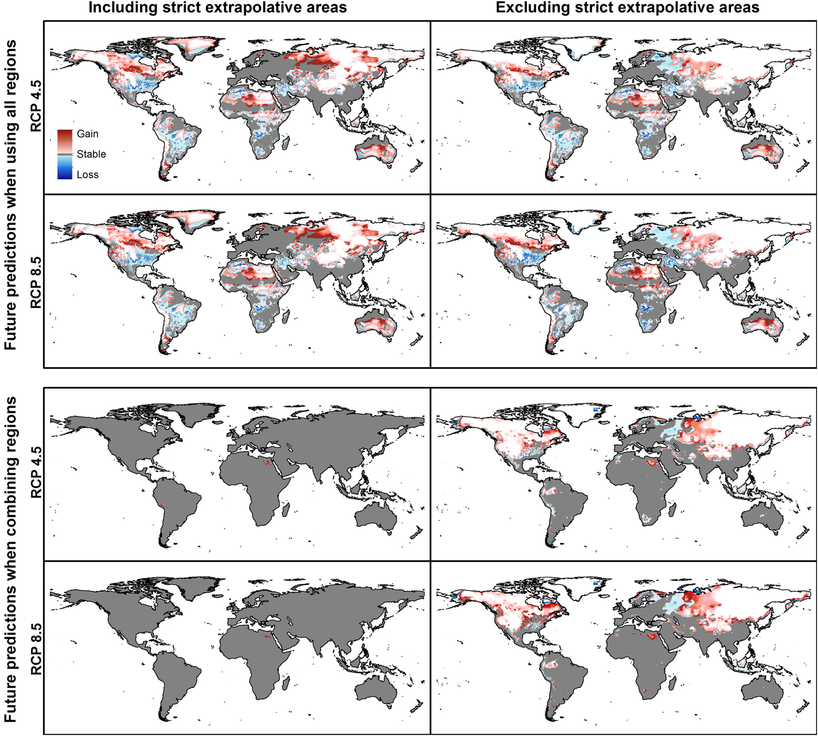
Summary of predictions for Rhipicephalus sanguineus sensu lato when models are created with data from all regions together and when models are created with each region and their results combined. Implications of including or excluding areas of strict extrapolation are shown for the two cases.
To contribute to the understanding of distributional ecology of species, it is crucial to characterize their environmental requirements, which in turn can inform about their geographic potential (Escobar and Craft, 2016). This study is the first to map the potential distribution and associated model uncertainty for the vector tick R. sanguineus sensu lato under both present and future conditions. Previous studies focused on the potential distribution of tick species, such as Amblyomma americanum (Raghavan et al., 2019b), Ixodes ricinus (Alkishe et al., 2017; Porretta et al., 2013), I. scapularis (Peterson and Raghavan, 2017a, b), and I. pacificus (Eisen et al., 2016, 2018). Although some of them identified extrapolative areas as a measure of uncertainty (Alkishe et al., 2017; Raghavan et al., 2019b), among-model variation from distinct sources has not been explored.
Although domestic dogs are the main host of Rhipicephalus sanguineus sensu lato, this tick species can use other domestic and wild hosts such as cats, birds, rodents, and humans (Dantas-Torres, 2010a). Based on this ability of using wide range of hosts, we did not include any host parameters in our models because collecting good-quality occurrence data for large numerous numbers of host species is not easy, and because it is not clear how one would best incorporate such data into these analyses.
Implications of pre-modeling processesResults of cleaning processes of data showed that multiple types of errors can reduce sample sizes considerably (of 9363 initial points, only 368 were kept for analyses). As model uncertainty depended importantly on the data we used, data cleaning procedures must be considered a crucial part of pre-modeling exercises (Cobos et al., 2018). Evidence of niche differentiation across the various distributional areas of the species was mixed considering the two methods used; when tested in geographic space, it resulted in more cases of rejection of niche similarity than when tested in environmental space (Table 3). This fact alerts us to cautions about use of single methods to test this aspect; more importantly, it informs us that this species’ niche could be broader than it is thought, which is common in invasive species (Jeschke and Strayer, 2008). Representations of the environmental space used and available for the species (e.g., Fig. 2) demonstrated a useful complement to results from the niche similarity tests.
Global and consensus distributional potentialResults from model predictions under future scenarios show new suitable areas in the Northern Hemisphere that were not identified as suitable under present conditions. These predictions should be treated with caution since these areas coincide with elevated (areas of extrapolation and high variation among models)(Figs. 4,5,6,7). These results concur with previous findings anticipating shifts of tick distributions towards more temperate areas (Alkishe et al., 2017; Raghavan et al., 2019b). Using multiple GCMs allowed us to capture a range of possible projections (Porfirio et al., 2014). Agreement of predictions among GCMs illustrates what to expect with different levels of certainty regarding changes in this species’ distribution. Using distinct GCMs and showing their agreement in prediction is still not a common practice in ENM [e.g., (Campbell et al., 2015; Raghavan et al., 2019b); however, we highlight the usefulness that this element has for interpreting results (Figs. 4,5,6,7).
As regards of models created with the dataset for all calibration areas versus results from the consensus of models created in distinct calibration areas, we observed more similarities in current than in future predictions. The main difference was that results from the consensus model included arid zones (deserts) and wet areas (tropical places in Amazonia and Africa) that were not part of the species’ potential distribution estimated from models created with all data (Figs. 3 and 7). This factor is intriguing as arid places are likely not adequate for this species’ development considering its need for humidity as other members of this group (Gray et al., 2013), but also because of exclusion of wet areas which may be thought to be suitable. More importantly, in future transfers, model created with all data predicted loss of suitability in areas expected to increase in humidity and temperature (Stocker et al., 2013), whereas the one resulted from consensus of regional models predicted stable suitability.
Implications of model uncertaintyIdentifying areas with high associated uncertainty in model projections is crucial to giving a clear picture and avoiding misinterpretations of the potential distributions of disease vectors (Peterson et al., 2011). However, projecting models into the future and interpreting those projections is not easy because such predictions include many and multifactorial sources of variation and uncertainty. We worked with numerous outputs from different climate models, emissions scenarios, model parameter settings, and model replicates. Using MOP analysis to identify areas with strict extrapolation risks and using hierarchical partitioning analysis and mapping to assess magnitudes, sources, and patterns of variation from the different sources are key approaches in this regard. For instance, our results indicated that amount and patterns of variation can change considerably depending on the data used to create models and the source of variation considered.
As regards of model variability, in contrast to previous results (Peterson et al., 2018), we found that the largest source of variation was replicates, followed by parameters, GCMs, and RCPs (Figs. 5 and 6). In accord with the previous results (Peterson et al., 2018), however, the minor contribution of RCP, compared to GCMs and replicates, points to methodological concerns as dominant rather than real-world consequences of different levels of greenhouse gas emissions. Extrapolation risk analyses (via the MOP metric) showed that interpretation of predictions in areas of strict extrapolation in model transfers could lead to erroneous or inadvisable conclusions (Owens et al., 2013). That is, the physiological response of the species in those areas is unknown; therefore, we have to be cautious about assuming that a species could potentially establish populations or not in such environmental conditions.
ENM results are also useful in understanding physiological tolerances of species, which, together with knowledge about ecology, behavior, and life history, can help to choose the most realistic predictions (Escobar and Craft, 2016). Global temperature increases are already affecting R. sanguineus sensu lato populations, which causes great concern regarding transmission risks of pathogens to humans and associated animals in temperate regions (Dantas-Torres, 2010b). For instance, MSF cases in Italy, southern France, Spain, and Portugal, peaked in 1980s and 1990s, but then decreased in the 2000s (Herrador et al., 2017); however, the reasons for this variation remain unknown. Hence, more information is needed to complement current information about this tick’s potential distribution, to design effective plans for preventing and mitigating risks.
The ability of R. sanguineus sensu lato to adapt to different environments, to complete its life cycle outdoors and indoors, and its potential to transmit the etiological agents of canine monocytic ehrlichiosis, MSF, RMSF, and canine babesiosis, make it an interesting and dangerous disease vector (Dantas-Torres, 2008). Our maps for current and future global potential distribution of this tick can help in understanding disease risk areas associated with this vector. Assessing uncertainty in model predictions is, however, of special importance for researchers and public health decision-makers. Before establishing any program, knowing which model outputs have the highest confidence versus which ones have higher uncertainty is crucial.
Authors’ contributionsAAA, and AMS provided the data for analysis. ATP, AAA, MEC, and AMS designed the experiments. MEC and AAA performed experiments, and produced figures and tables. AAA, MEC, and ATP wrote the manuscript. All authors revised and approved the manuscript.
Availability of data and materialsAvailable.
Consent for publicationNot applicable.
Ethics approval and consent to participateNot applicable.
Competing interestsThe authors declare that they have no competing interests.
FundingAAA was supported by the Ministry of Higher Education, Libya. AMS was supported by the Graduate Fulbright Egyptian Mission Program (EFMP).
The authors would like to thank the University of Kansas Ecological Niche Modeling (KUENM) Group. Thanks to the Ministry of Higher Education, Libya, for supporting AAA during his studies at the University of Kansas. Special thanks to the staff of the Zoology Department, Faculty of Science, University of Tripoli, Tripoli, Libya, for their continuous support during the study. Alkishe thanks Amel Dwebi for her support and encouragement during this work.
The following are Supplementary data to this article: