


Unlike species with widespread distributions, few predictive models have been constructed for species with restricted or unknown distributions. One example of such a poorly studied species is Aristolochia gigantea, for which very conflicting information has been reported regarding its distribution. In this study, we present A. gigantea's distribution and range, the environmental factors responsible for its distribution and comments about the information available in the existing literature. The model of A. gigantea's distribution identified new areas that can be surveyed to potentially find new populations, and our results reinforce the importance of predictive models for studying the distributions of species, suggesting that ecological niche modeling can provide important contributions to the analysis of biogeographic patterns in little-studied plant species.
Conservation practices typically utilize information on species that are endemic or restricted to certain areas, or even the richness of higher taxa, to identify priority areas for conservation (van Jaarsveld et al., 1998). Thus, information on the distribution and range of focal species and an understanding of their biology are extremely important.
The analysis of the geographic distribution patterns of various taxa and at different spatial scales has increased in recent years (Guisan and Thuiller, 2005; Jiménez-Valverde et al., 2008). Among the tools used for this type of analysis, the most attention has focused on predictive species distribution models, in which the potential ecological niche of a species is modeled from various hypotheses as to how environmental factors control the distribution of species and communities based on known occurrence points (Guisan and Zimmermann, 2000). Such techniques are based on the fundamental niche concept proposed by Hutchinson (1957), which represents a niche as a range of conditions and resources in a hyper-volumetric space that is potentially exploitable by a species, disregarding biotic interactions with other species.
In general, spatial modeling converts primary occurrence data in the form of species records into geographic distribution maps that indicate the likely presence or absence of a species (Araújo and Guisan, 2006). The algorithms used for such conversions attempt to establish non-random relationships between the presence/absence data and the environmental variables relevant to the species (e.g., temperature, rainfall, topography, etc.).
Unlike with widely distributed species, few models have been applied to rare species considered here as those having low abundance and/or small ranges (according to Gaston, 1994); this is because their occurrence records are generally scarce and sometimes lacking data accuracy (Engler et al., 2004; Siqueira et al., 2009) due to small geographic distributions, low abundances or insufficient collecting. However, the application of the modeling technique utilized here is very useful in characterizing geographic distributions based on often-incomplete datasets, as with species for which little information is available and that may have errors in their reported distribution (Siqueira et al., 2009).
One example of a poorly studied species is Aristolochia gigantea Mart & Zucc, a basal angiosperm that, within the genus to which it belongs, is the most widely cultivated for ornamental purposes (Lorenzi and Matos, 2002), most likely due to the lack of a foul odor in this species. Natural populations of this species in Chapada Diamantina evidenced moderate to low levels of intra-population genetic variability, probably due restricted distribution of the species and small population sizes (Hipólito et al., 2012).
The first description of A. gigantea with details regarding species distribution comes from the work of Martius and Zuccarini (1824), and its natural distribution was reported in the state of Bahia, Brazil in the habitat in fences near the mountains of Jacobina that are in a desert place. Masters (1869) complemented that the plant is assigned to “mountainous” locations in Bahia and Minas Gerais, followed by Bellair and Saint-Leger (1899), who assign the origin only to Bahia; and Rodigas (1893), Costa and Hime (1981) and Capellari-Junior (1991) assign the origin to Bahia and Minas Gerais. Different information can be found in Barringer (1983) that recorded the occurrence of the plant in the rainforests of Panama and the Brazilian Amazon, although the author reports differences in the material from Central America and from South America, with larger flowers in the latter.
According to Capellari-Junior (1991), this species occurs in regions of the Caatinga biome, prefers damp areas such as riverbanks, secondary forests, pastures and road edges, and when cultivated, grows well in any soil. Its adaptability may explain the confusion regarding the origin of the species, e.g., the population reported by Barringer (1983) in the Amazon, which, according to Capellari-Junior (1991), likely originated from cultivated stock.
Herbarium records indicate that A. gigantea populations have also been found in several additional sites, including the Brazilian states of São Paulo, Rio de Janeiro, Santa Catarina and Paraná and outside of Brazil in Costa Rica, Panama and the United States. In some of these herbarium records, additional information is included on the occurrence of the species, such as whether it was natural or cultivated, but in others, this information is lacking, complicating the circumscription of the natural range of the species.
Thus, due to the inconsistency of the information available for this species coupled with the need for knowledge of the species’ distribution, it is necessary to clarify the distribution of A. gigantea. In this context, this paper aims to (1) describe the distribution of A. gigantea and compare it in different models, (2) analyze whether there is an association between the species’ predicted distribution of the species and the sites in which it is found, (3) evaluate the environmental factors responsible for determining the species’ distribution limits, (4) analyze whether there is an association between the distribution and the information on this species reported in the literature and for all these aims to (5) explore the issue of using predictive species distribution models as a tool to perform or improve the assessment of unknown distribution species.
Material and methodsStudy areaBecause the natural distribution of A. gigantea is uncertain, we chose to construct distribution maps in two steps. The first step considered fine scale distribution maps with the goals of increasing the distribution model's accuracy and restricting predictions to the most likely occurrence limits and at the second step we aimed to indicate possible new areas of occurrence since no certainty exists about its natural occurrence.
Thus the first distribution maps included information found in older records commonly found in the literature, which name Bahia (BA) (Martius and Zuccarini, 1824; Bellair and Saint-Leger, 1899) and Minas Gerais (MG) (Masters, 1869; Rodigas, 1893; Costa and Hime, 1981; Capellari-Junior, 1991) as the areas of its natural occurrence. In addition, at the second step of distribution mapping we included the entire Brazil country.
Data collectionTo model the potential geographic distribution of A. gigantea, we decided to combine historical herbarium records with recent field records. These points came from the region surrounding Chapada Diamantina, Bahia, totaling fifteen occurrence records from five different municipalities (Morro do Chapéu, Utinga, Lençóis, Itaetê and Rio de Contas). These records were obtained through active and systematic searches of the Chapada Diamantina region and nearby locations, with pursuits focused on areas close to small water bodies. The geographical coordinates of each location were recorded with the aid of a GPS unit, at points very close to where individuals were observed or in the approximate center of a population.
Other occurrence points were obtained from herbarium records and through the Species Link page (distributed information system that integrates primary data from biological collections URL: http://splink.cria.org.br/). Records containing information from cultivated species or doubtful identification, as some specimens from Panama as probably Aristolochia braziliensis were excluded from analyses. We also excluded duplicate instances and data with incomplete information, i.e. without coordinates or city information. A total of 94 presence records were obtained (including those obtained in the field) (Fig. 1).

Absence records data from different locations in Chapada Diamantina, Bahia were obtained at the same areas where systematic searches were made (as pointed before); we added thus information about 45 absence records.
Selection of environmental variablesAs studies of lianas are not frequent in the literature, the selection of environmental variables was based on the general physiological ecology of plant species, considering aspects of water dependency, interfaces with other physiognomies and geomorphological and topographic factors (Guarino and Walter, 2005).
Based on those considerations, we opted to include the following variables: soil drainage and fertility; the cation exchange capacity of soils; altitude (elevation above sea level); mean diurnal range; temperature seasonality; mean temperature of warmest quarter; precipitation of wettest month; precipitation of warmest quarter; precipitation in the wettest quarter; precipitation in the driest quarter; annual mean temperature; maximum temperature in the warmest month; minimum temperature in the coldest month; annual precipitation; temperature seasonality, mean temperature of warmest quarter, precipitation of wettest month and precipitation of warmest quarter.
The bioclimatic variables were obtained from the WorldClim Project (Hijmans et al., 2005) in the form of grids with a spatial resolution of 30 arc seconds (approximately 1km). Digital models of vegetation, drainage and soil fertility were obtained from the website of Embrapa Solos (available at http://mapoteca.cnps.embrapa.br/geoacervo) at a scale of 1:5,000,000 and were adjusted to a resolution of approximately 900m for comparison with the other variables; further data were acquired from the World Soil Information portal (available at http://www.isric.org/). Finally, the topographic variables were obtained from the website of the “Shuttle Radar Topography Mission” (SRTM) (available at http://www.worldclim.org/current.htm) and had a spatial resolution of 30 arc seconds.
To test for correlations (Pearson correlation coefficient>0.70) between predictor variables, 1000 random points were created in Bahia and Minas Gerais in ArcGis and environmental variables were extracted to be tested. Some variables were thus excluded from analyses: precipitation in the wettest quarter; precipitation in the driest quarter; annual mean temperature; maximum temperature in the warmest month; minimum temperature in the coldest month; and annual precipitation because they were too correlated. Same selected variables were used in all models (below).
Generation of modelsAs different models can be used in species distribution modeling we choose to use more them one model to predict A. gigantea range and thus we contrasted the models based on evaluation of each one. In that manner, we could choose the most parsimonious model for a broader application and results.
The first model used was the MaxEnt (Maximum Entropy) algorithm version 3.3.1, which, through an optimization process, predicts the likelihood of species to occur in a geographic area subject to the constrain that the expected value of each environmental variable under this estimated distribution matches its empirical average (Phillips et al., 2006).
Maxent was analyzed by jackknife test of variable importance to access the contribution of each variable alone and coupled with others and bootstrapping manipulations using 75% for training and 25% for validation, with 100 replications.
Since we have not only presence data but also absences, models of logistic regression are also interesting and maybe more close to real species distribution occurrence. Thus, we used the generalized linear model (GLM) with the binomial link family to compare models using R software (version 3.0.2, bbmle package). We used the Akaike's criteria (AIC), and the derived parameters AICc, ΔAICc and wAICc, to get the best combination of predictors for the regression model.
Model evaluationTo evaluate models consistency and select the best model of each distribution model we used the same independent validation data which consisted of 20 sorted points of presences (10) and absences (10) of A. gigantea that were not used to generate the models and plot them on the probability of presence maps of GLM and MAXENT. The map of GLM was given by: p=1/1+e−[f(x)]; where function f represents the best logistic model. Points were thus observed on maps to visual analyses and we performed a kappa test for quantitative analyses.
To assess the quality of the generated distribution models, an analysis of the “receiver operating characteristic curve” (ROC) was performed, which evaluates the performance of the model using a single value representing the area under the curve (AUC).
The successes of the three models were compared by analyzing their goodness in fitting their predicted presence and absence probabilities and the validation data by thresholds through kappa statistics, a test similar to accuracy but that takes into account the proportion of correct predictions expected by chance. We arbitrarily selected 80% as the threshold for the presence probability and reclassified the distribution map into two classes (presence>80%, and absence<80%).
ResultsModels generated to A. gigantea distribution in Bahia and Minas Gerais evidenced average AUC above 0.9 (Maxent=0.924; GLM=0.967). Maps evidenced great differences (Fig. 2) that revealed the best performance from GLM model, as also evidenced by kappa statistics (Maxent: observed agreement=0.55; k=0.1; p=0.1525; GLM: observed agreement 0.95; k=0.9; p<0.0001).

Models generated for Brazil (Fig. 3) evidence the similar pattern that was obtained by Bahia and Minas Gerais prevision, and the map also evidenced AUC above 0.9 (Maxent=0.974) and best performance from GLM model in kappa statistics (Maxent: observed agreement=0.7; k=0.4; p=0.0127; GLM: observed agreement 0.95; k=0.9; p<0.0001).

In Bahia and Minas Gerais maps generated by Maxent evidenced a limited occurrence range (Fig. 2) and tended to create more omission errors, i.e. tended to consider that the plant is in a place where naturally it does not occur, these were more clear when we transformed the map in only presences and absences probabilities (Fig. 4). Meanwhile, maps generated by GLM evidenced a larger distribution for the species and the transformed map for presences and absences produced apparently a more reliable data as only one error was measured (Fig. 4). In Brazil maps, models performed in the same manner as in Bahia and Minas Gerais maps (Fig. 4).
 are based on GLM model and figures below (c and d) on Maxent model.")
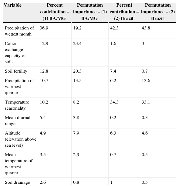
Explaining variables that were used to generate models differed between maps. The variable that best explains the models generated for Bahia and Minas Gerais in Maxent model was the Precipitation of Wettest Month (with 36.9% of contribution), however in permutation importance, the model was best explained by the cation exchange capacity of soils (23.4) even with a lower contribution (12.9%) (Table 1). The variable Precipitation of Wettest Month also had the higher percent contribution (42.3%) in Brazil distribution but at this model, this variable also evidenced a higher permutation importance (43.8) (Table 1).
Maxent contribution variables in two different models for A. gigantea distribution modeling (1) Bahia and Minas Gerais (BA/MG) and (2) Brazil. Values are ranked based on BA/MG crescent contribution.
| Variable | Percent contribution – (1) BA/MG | Permutation importance – (1) BA/MG | Percent contribution – (2) Brazil | Permutation importance – (2) Brazil |
|---|---|---|---|---|
| Precipitation of wettest month | 36.9 | 19.2 | 42.3 | 43.8 |
| Cation exchange capacity of soils | 12.9 | 23.4 | 1.6 | 3 |
| Soil fertility | 12.8 | 20.3 | 7.4 | 0.7 |
| Precipitation of warmest quarter | 10.7 | 13.5 | 6.2 | 13.6 |
| Temperature seasonality | 10.2 | 8.2 | 34.3 | 33.1 |
| Mean diurnal range | 5.4 | 3.8 | 0.2 | 0.3 |
| Altitude (elevation above sea level) | 4.9 | 7.9 | 6.3 | 4.6 |
| Mean temperature of warmest quarter | 3.5 | 2.9 | 0.7 | 0.5 |
| Soil drainage | 2.6 | 0.8 | 1 | 0.5 |
Models generated by GLM evidenced a major contribution by the combination of temperature precipitation of wettest month and altitude (dAICc=0; df=5; weight=0.57).
DiscussionAlthough Maxent models have demonstrated better performance with small datasets compared with other methods such as SVM (support vector machines) or GARP (genetic algorithm for rule-set production) in other cases (Elith et al., 2006), in this study GLM model was the best predictor and evidenced results very different from those generated by Maxent.
The GLM map (Fig. 2) demonstrated that A. gigantea distribution should be greater than the sampled yet. This map could also support the hypothesis that the species has its origins in both states (Bahia and Minas Gerais) and thus increases the strength of the species description that attributes its origin to theses states decreasing theories about its origin outside these states.
In order to compare preferential biomes for species based on literature references, we overlapped WWF biomes maps with our predicted models (Maxent and GLM models). Maps evidenced preferential areas of Atlantic dry forest and Caatinga in Maxent model and beyond these areas for Bahia interior forest and a small strip of Cerrado for GLM model. Despite some difference in Capellari-Junior's (1991) description, that attributed only Caatinga biome, differences in biomes were thus expected as Chapada Diamantina (where most occurrence points were found) is characterized by a mosaic of vegetation types (Neves and Conceição, 2007).
Our results may have suffered from bias caused by the number of points used for modeling, as we had only nine presence points in the state of Minas Gerais with no possibility of collecting more data from that state. However, during the analysis, we chose not to delete points in Bahia to balance model sample sizes, as fewer points may have further compromised model quality, as demonstrated previously by Hernandez et al. (2006), who showed that the ideal is to use at least 50 occurrence points for MaxEnt modeling.
Lower collection effort in Minas Gerais increases the need for expeditions to areas where there are few or no register of natural species records to validate the model, including increasing the collection effort in this state. Preferably, areas for collects should include Atlantic dry forest areas, south areas of Caatinga biome in Brazil and Bahia interior forest. Searches in Cerrado areas could increase accuracy in model, probably through absence of natural populations in this biome (as the prediction in this area was too restricted).
Absence of populations from predicted presence locations, as evidenced in GLM map (Fig. 2), could be explained (among other theories) by the extinction of intermediate populations due to geographic barriers or the decrease in number of natural populations through gene erosion combined with low effective pollination and its reproductive dependence on biotic vectors with small fly range (Hipólito et al., 2012). Although, alternative explanations can go on the other hand, as the presence of actually natural populations (considered as those in natural places with no directly human interference) could be once long distant dispersed trough human interference as Capellari-Junior (1991) point out about its ease capacity of cultivation in different locations and causing false natural locations.
Although Brazil distribution maps evidenced higher AUC values and an excellent performance in kappa statistics, these maps can suggest only that the species could survive and can form natural population's through dispersion in Southeast and South Brazil. Data should be seen carefully however as there are more points in Bahia and Minas Gerais specially on the first due to increased collection efforts.
Other data that should be seen carefully refer to the environmental factors responsible for determining the species distribution limits. In general, the species showed tolerance limits to temperature and precipitation although differences in Maxent and GLM models. We evidenced the need for more information on biological data from species to assume reliable modeling predictions especially for Aristolochia gigantea where this kind of data is too scarce.
Combining historical herbarium records with recent field records provides an opportunity to illustrate how knowledge of the distribution of a species can be refined and understood for conservation purposes with contemporary field surveys. Different algorithms used to generate the models also evidenced the need to calibrate the model through reliable field data obtained before and tested after model predictions.
The results of the present study reinforce the importance of predictive models for the study of species distributions, suggesting that ecological niche modeling can provide important contributions to the analysis of biogeographic patterns and processes related to poorly studied plant species. Conservation practices should take into account the increased amount of information available for the species, including its distribution and requirements for maintaining populations.
Conflicts of interestThe authors declare no conflicts of interest.
We thank the assistance for their contribution with plant collection, CAPES for a scholarship granted to J. Hipólito through the Graduate Program of Pós Graduação em Ecologia e Biomonitoramento (UFBA), CNPq for a scholarship in productivity research to B.F. Viana and financial assistance for the research. We also thank UFBA for enable the English revision of the manuscript.

